VODACOM Business Nigeria has said that technology can help small and
medium enterprises adapt to market changes, increase productivity, and
improve competitive advantage.
Sharing insights on this possibility recently at the NigeriaCom 2015,
CIO Forum, Vodacom’s Executive Head of products and services, Wale
Odeyemi, said that one of the most important benefits of unified
communications for SMEs is that customers can access the network from
multiple devices at the same time.
This makes it easy to manage contacts, send and receive voice over
internet protocol (VoIP) calls and carry out multiple communications at
the same time, which enables video conferencing to take place on a
laptop while a voice call takes place on a worker’s mobile phone.
Business employees
Odeyemi revealed that 75% of small business employees say that
flexible working has made them more productive. According to Odeyemi,
productivity gains are one of the many reasons for SMEs to take
advantage of unified communications. Other gains include cost reduction,
increased customer service and improved competitive advantage.
He explained that from instant messaging features to using the
internet for voice calls unified communications improves profit
margins by boosting overall operational efficiency; this is especially
true for businesses that have mobile employees.
Friday, 25 September 2015
Samsung raises bar in home experience with Activ dualwash
While technology evolves,Samsung has continued to excite consumers
with something new particularly at the upper end of its ‘washing machine
line-up’.
This development has earned Samsung a reputation in the Nigerian market for its wide range of top quality home appliances and hand-held devices, including, smartphones and Ultra High Definition televisions.
This year, the company has again raised the bar in home experience with the introduction of more traditional and professionally-inspired Activ dualwash, with smart built-in sink, water jet, magic filter and dispenser, with a warranty of 10 years.
Understanding consumer constraints in washing, the Activ dualwash cares for not only the clothes, but also the homemaker.
The product, a first of its kind with a built-in sink is designed to elevate the everyday home experience for consumers, making laundry at home easier and even providing health benefits.
The Activ dualwash is a result of years of research to improve the time and energy spent doing laundry.
Unique attraction
The Activ dualwash is uniquely and innovatively designed with a built-in sink with water jet and a gentle scrubbing surface. This all-in-one solution saves time, reduces effort and avoids mess by enabling consumers to presoak, scrub and auto wash the entire wash process in the washing machine, instead of having to spread the process over multiple locations, giving users more time to do other important things.
Benefits
The Activ dualwash system comes with a dedicated sink that provides a convenient space to soak and/or hand-wash delicate items and comfortably pre-treat heavily stained areas of clothes before starting a normal wash cycle. The water jet, which starts and stops at the push of a button, provides access to water, thus allowing for easy soaking and scrubbing. Once that is done, the laundry and water can easily be poured into the machine by simply lifting the sink. This drops the items into the tub below for a spotless wash that completes the effortless, all-in-one washing process.
Magic dispenser
The magic dispenser eliminates residual detergent on fabric, leaving users with clean and fresh clothes. It achieves this by creating a powerful water vortex that dissolves detergent and disperses it completely, thoroughly and evenly before the wash cycle starts. Washing has never been better!
Magic filter
The Magic Filter is a long and wide filter, located at the tub’s water level. It takes care of the details that make clothes look fresh and clean. It keeps unwelcome specks off whites and darks by gathering lint, fluff and particles, so you can look good without having to inspect and tidy the little things. It does all this while protecting your drain from getting clogged.
Wobble technology
The product utilises Samsung’s revolutionary Wobble technology, which helps to protect delicate fabrics from friction damage without compromising the washing performance. State-of-the-art wobble pulsators generate a dynamic, multi-directional washing flow that prevents tangles, twists and knots while thoroughly cleaning your clothes with increased washing power that requires less water consumption. Ironing has been made easy for users as the fabric comes out with less tangling.
Rear control panel
Located at the back of the machine, the Rear Control Panel provides better visibility and ease of use while also being protected from water splashes during hand and pre-washing. The panel’s dual cluster design clearly separates the control buttons so that they are much simpler to learn and use.
With the Smart Check automatic error-monitoring system, there is absolutely no need to refer to paper manuals any more as it can detect and diagnose problems, using a smartphone app.
Design
The Samsung Activ dualwash is uniquely designed, with a naturally rounded and elegant curves, an LED display, a strong and durable tempered glass door and a smart functionality with remote monitoring system.
Bottom-line
The Samsung Activ dualwash washing machine is synonymous with innovation and sleek design, making it the first and the best digital washing technology available without compromising on style.
Not only does it deliver incredible speed and accuracy through advanced washing features, it is durable, works smart and users can trust it.
The Activ dualwash has been engineered to offer superior washing experience while maximizing simplicity and ensuring that users are just one click away from seamless laundry – definitely a must-have for the homemaker concerned with optimising her time.
4bn people lack internet access as global broadband grows slowly
The United Nation Broadband Commission, Monday disclosed that four
billion people globally, especially people living in the developing
world lack internet access, just as broadband grows slowly.
The UN, in its 2015 report stated that the new country by country data on state of broadband access worldwide is published by the UN Broadband Commission.
Released just ahead of the forthcoming SDG Summit in New York and the parallel meeting of the Broadband Commission for Sustainable Development on September 26, the report further revealed that 57% of the world’s people remain offline and unable to take advantage of the enormous economic and social benefits the Internet can offer.
The lowest levels of Internet access, according to the report are mostly found in sub-Saharan Africa, with internet available to less than 2% of the population in Guinea (1.7%), Somalia (1.6%), Burundi (1.4%), Timor Leste (1.1%) and Eritrea (1.0).
New figures in the report confirmed that 3.2 billion people are now connected, up from 2.9 billion last year and equating to 43% of the global population.
But while access to the internet is approaching saturation levels in the developed world, the net, according the study is only accessible to 35% of people in developing countries.
The situation in the 48 UN-designated Least Developed Countries is particularly critical, with over 90% of people without any kind of internet connectivity.
Accordingly, the report showed that the top ten countries for household Internet penetration are all located in Asia or the Middle East.
While the Republic of Korea continues to have the world’s highest household broadband penetration, with 98.5% of homes connected; Qatar (98%) and Saudi Arabia (94%) are ranked second and third respectively.
Iceland, according to the report has the highest percentage of individuals using the Internet (98.2%), just ahead of near-neighbours Norway (96.3%) and Denmark (96%).
Monaco remains very slightly ahead of Switzerland as the world leader in fixed broadband penetration, at over 46.8% of the population compared with the Swiss figure of 46%.
According to the report, there are now six economies including Monaco, Switzerland, Denmark, Netherlands, Liechtenstein and France where fixed broadband penetration exceeds 40%, up from just one (Switzerland) in 2013.
The Asia-Pacific region, the report indicated now accounts for half of all active mobile broadband subscriptions, with Macao, China easily taking top place with 322 active mobile broadband subscriptions per 100 people or just over 3 subscriptions per inhabitant followed by second-ranked Singapore (156 subscriptions per 100 people) and Kuwait (140 subscriptions per 100 people).
In total, there are now 79 countries where over 50% of the population is online, up from 77 in 2014. The top ten countries for Internet use are all located in Europe.
With the 17 goals now firmly on the global agenda, governments and private industry both have a strong interest in finding ways to get people online, the report argues, the report added.
“The UN Sustainable Development Goals remind us that we need to measure global development by the number of those being left behind,” ITU Secretary-General Houlin Zhao, who serves as co-Vice Chair of the Commission with UNESCO Director-General Irina Bokova., said, adding that, “The market has done its work connecting the world’s wealthier nations, where a strong business case for network roll-out can easily be made. Our important challenge now is to find ways of getting online the four billion people who still lack the benefits of Internet connectivity, and this will be a primary focus of the Broadband Commission going forward.”
“The 2030 Agenda recognizes the power of new technologies to accelerate human progress, to bridge the digital divide, to develop knowledge societies – we must do everything to support States in reaching these goals, especially developing States,” , the UNESCO Director-General, Irina Bokova, said, adding that, “This calls for stronger efforts by governments and all actors, in ensuring access, use and affordability – it requires also greater work to build the capacities of all women and men to make the most of all new opportunities.”
Produced annually by the Broadband Commission, the State of Broadband is a unique global snapshot of broadband network access and affordability, with country-by country data measuring broadband access against key advocacy targets set by the Commission in 2011.
Broadband Internet, according to the new report is failing to reach those who could benefit most, with Internet access reaching near-saturation in the world’s rich nations but not advancing fast enough to benefit the billions of people living in the developing world.
The State of Broadband 2015 is the fourth edition of the Commission’s broadband connectivity report. Released annually, it is the only report that features country-by-country rankings based on access and affordability for over 160 economies worldwide.
The Broadband Commission comprises more than 50 leaders from across a range of government and industry sectors who are committed to actively assisting countries, UN experts and NGO teams to fully leverage the huge potential of ICTs to drive new national SDG strategies in key areas like education, healthcare and environmental management.
Phase3 to increase investment on infrastructure for network services
Independent fibre optic infrastructure and telecommunications
services provider, Phase3 Telecom has said it will deepen investment on
infrastructure to extend its reach, increase efficiency, scale up
resilience and adaptability for efficient network services while
offering solutions that will amplify the operations of its clients
across the West African sub-region.
The Chief Executive Officer of the company, Mr Stanley Jegede said the firm will continue invest on robust network to enable the firm extend its reach as the IT world migrates to the new era of internet of things (IoT).
“As more clients that ride on Phase3 network take advantage of the Internet of Things to deliver efficiency in their areas of business; it is very important for us to continue to extend reach as well as adopt the best technology and resource to make our network more secure, resilient and adaptive. Without this, the network will be largely exposed to incessant point of failure with fatal impact on the client and huge cost in millions on downtime.”, he said.
Jegede added that the focus of Phase3 in the coming months; is not just to drive a network infrastructure that connects people but to be the frontrunner in scaling a network that helps grow economies and effectively support technological innovations that expand the world and make it better in all sectors.
This is essential to accelerating the social development, growth in gross domestic product (GDP) and productivity the sub-region has been clamoring for.
The firm which is set to mark its 12th year anniversary next month, said because of its capacity to deliver homegrown solutions deliver significant long term value and as part of its wider West Africa roll out plan to deliver regional connectivity through a single network, it has commenced the deployment of a 228 km long aerial fiber optic infrastructure from Kano to Gazaoua in the Republic of Niger, a landlocked country that borders six other countries of Algeria, Benin, Burkina Faso, Chad, Libya and Mali.
The project is under the Niger-Nigeria fiber-optic cable project being facilitated by the Universal Service Provision Fund (USPF) through the extension of the Backbone Transmission Infrastructure Programme (BTRAIN) programme.
Being an indigenous firm, Phase 3 has been at the forefront of increasing backbone infrastructure that will boost digital market viability and minimise the challenges of accessibility and reliability across sectors and layered connectivity needs
Truemessenger: Tackling spam SMS menace to make SIM smarter
The penetration of mobile instant messaging platforms such as
Whatsapp, Black Berry Messenger (BBM), Palmchat, 2go, among others in
Nigeria’s social media ecosystem has no doubt increased appreciably.
But despite this deep penetration, Short Message Service (SMS), also known as ‘text message’ and the oldest instant messaging platform, still remains relevant.
Reasons: While the other instant messaging platforms run only on smart phones and are internet-enabled, SMS requires no internet and as such it runs on both smart and non-smart phones.
While smart phone usage in Nigeria is on the increase by April, 2015, global Personal Computer (PC) firm, Lenovo revealed that the Smartphone penetration in Nigeria had reached the 30 percent mark, thus making Nigeria one of the fastest growing smartphone markets in the world, with Android being the most widely used operating system in Nigeria.
Data available from StatCounter appears to support Lenovo’s finding. According to the data, Android usage increased by about 19 per cent within a year from 10.95% in August 2013 to 29.94% in August 2014; and it is still growing.
Similarly, statistics from the Monthly Subscriber Data of the Nigerian Communications Commission (NCC), the country’s telecom regulatory authority, puts Nigeria’s tele-density at 100.59 per cent as of the end of January 2015, with active lines/phone numbers on the telecommunications operators’ networks reaching 140,822,483 and 146 million as at April 2015.
With such a massive subscription base, coupled with the increasing usage of Android smart phones, and directive by the NCC that all mobile network operators should charge a flat rate of N4 per SMS to other Nigerian networks, one can conclude that SMS no doubt, a viable and effective medium for reaching a large number of Nigerians with various messages at a cheap rate.
However available statistics show that, spam messages account for 15 per cent of all SMS messages sent globally, representing 1.2 trillion spam messages each year.
The implication of this is that vast majority of mobile subscribers, most of who fall within the category of smart phone users, are now at the mercies of marketing outfits and even fraudsters who reach out to their targets via the SMS.
This development has continued to worry both the subscribers and the regulatory agencies. Every second for instance, mobile subscribers in Nigeria are bombarded with text messages that are of little or no interest to them from their network provider.
Thus spam SMS has become a matter of serious concern to subscribers looking for possible solution to get a way with it.
But with the latest app from Truecaller, a leading search technology company, there are positive signals that telecoms subscriber will have a relief .
In what seems like a response to these yearnings, recently launched Truemessenger, a revolutionary app which aims to take care of spam and make the SMS experience smarter and more social.
Speaking about the new App and its unique functions, Alan Mamedi, CEO& Co-founder of Truecaller explained that the introduction was necessitated by the urgent need to tackle the menace which spam messages have become to mobile network subscribers not just in Nigeria but all over the world.
Mamedi said, “We are at a crossroads of sorts, in terms of spam messages we receive on our mobile phones, and despite the evolution of services in other areas, little has been done to curb the number of spam messages we receive on a daily basis. Truemessenger aims to attacks this problem head-on by using a combined power of our global community with information from your own personal networks so you’ll never again have to worry about anonymous numbers.”
One of the unique features of the Truemessenger App is its ability to filter and block spam SMS by tapping into a vibrant community of more than 150 million members who help protect one another from annoying intrusions.
Explaining how the App functions, Mamedi said that Truemessenger organizes the inbox, puts a name to a number, and seamlessly blocks and filters spam SMS messages. It automatically checks incoming messages against the user’s contact list for pre-existing contact information and adds the name of the sender instead of showing the phone number. Thus mobile phone users now have the option of avoiding messages from unwanted numbers and contacts.
Another unique feature of the Truemessenger app is its ability to enable mobile phone users to establish SMS spam rules, a function that was only available on the email and filters spam out of inbox or totally block it thereby keeping the inbox clean. It also has the ability to pull information from social networks and automatically assigns photos, nicknames and other contact information to incoming text messages.
Interested mobile users can now download the Truemessenger on their Android, the only platform where it can run at the moment, from the Google App store for free. According to the owners Truemessenger is complementary to the Truecaller and Truedialer apps. But while the Truedialer is available for free on Android and Windows Phone, the Truecaller can be downloaded for free on popular platforms including Android, iOS, Windows Phone, BlackBerry, Tizen and Nokia feature phones.
Microsoft Corp, Monday, began the worldwide release of Office 2016,
delivering new versions of the Office desktop apps for Windows,
including Word, PowerPoint, Excel, Outlook, OneNote, Project, Visio and
Access. The apps are the latest addition to Office 365, Microsoft’s
cloud-based subscription service that help people do their best work,
together. Also launched were the new and enhanced Office 365 services
built for team productivity.
 “The way people work has changed dramatically, and that’s why
Microsoft is focused on reinventing productivity and business processes
for the mobile-first, cloud-first world,” Satya Nadella, chief executive
officer of Microsoft, said, adding that, “These latest innovations take
another big step forward in transforming Office from a familiar set of
individual productivity apps to a connected set of apps and services
designed for modern working, collaboration and teamwork.”
“The way people work has changed dramatically, and that’s why
Microsoft is focused on reinventing productivity and business processes
for the mobile-first, cloud-first world,” Satya Nadella, chief executive
officer of Microsoft, said, adding that, “These latest innovations take
another big step forward in transforming Office from a familiar set of
individual productivity apps to a connected set of apps and services
designed for modern working, collaboration and teamwork.”
Nadella wrote about the new Office on the Official Microsoft Blog. Corporate vice president for the Office Client Applications and Services team, Kirk Koenigsbauer provided more insights into Office 2016 on the Office Blog.
By subscribing to Office 365, customers can get always-up-to-date, fully installed apps for use across their devices, combined with a continually evolving set of consumer and commercial services, such as OneDrive online storage, Skype for Business, Delve, Yammer and enterprise-grade security features.
Together, the new Office and Windows 10 are the most complete solution for doing work. The Office 2016 apps run beautifully on the best Windows ever, including the new Sway for Windows 10 to create shareable, interactive stories that look great on any screen.
Features of the app includes: Windows Hello which logs you into Windows and Office 365 in one simple step.1 Office Mobile apps on Windows 10 empower on-the-go productivity, and work with Continuum2 so you can use your phone like a PC. Cortana3 connects with Office 365 to help with tasks such as meeting preparation, with Outlook integration coming in November.
Built for teamwork
*The Office 2016 apps simplify collaboration and remove barriers to team success. Co-authoring4 is now provided in Word, PowerPoint and OneNote desktop software, including real-time typing in Word that lets you see other peoples’ edits as they make them.
*Skype in-app integration across the rich client apps allows you to IM, screen share, talk or video chat right in your docs.
*Office 365 Groups are now an integrated part of the Outlook 2016 client app and available on your favorite mobile device through the Outlook Groups app, delivering a consistent team experience across the suite. In addition, a new Office 365 solutions that combine the power of apps and services for better collaboration are coming soon.
Introduced yesterday, Office 365 Planner helps teams organize their work, with the ability to create new plans, organize and assign tasks, set due dates, and update status with visual dashboards and email notifications. Planner will be available in preview to Office 365 First Release customers starting next quarter.
Significant new updates to OneDrive for Business are coming later this month, including a new sync client for Windows and Mac, which will deliver selective sync and enhanced reliability. Updates also include increased file size and volume limits per user, a new user interface in the browser, mobile enhancements, and new IT and developer features.
Unveiled earlier this year, GigJam is available Tuesday in private preview and will become part of Office 365 in 2016. GigJam is an unprecedented new way for teams to accomplish tasks and transform business processes by breaking down the barriers between devices, apps and people.
Availability and requirements
The new Office 2016 apps, according Microsoft are available in 40 languages and require Windows 7 or later. Starting yesterday, Office 365 subscribers can choose to download the new Office 2016 apps as part of their subscription. Automatic updates will begin rolling out to consumer and small-business subscribers next month, and to commercial customers early next year. Office 2016 is also available today as a one-time purchase for both PCs and Macs.
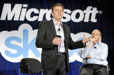
File:
Skype Chief Executive Tony Bates, left, Microsoft Chief Executive,Steve
Ballmer, at a news conference in San Francisco on the
acquisition:Reuters
Nadella wrote about the new Office on the Official Microsoft Blog. Corporate vice president for the Office Client Applications and Services team, Kirk Koenigsbauer provided more insights into Office 2016 on the Office Blog.
By subscribing to Office 365, customers can get always-up-to-date, fully installed apps for use across their devices, combined with a continually evolving set of consumer and commercial services, such as OneDrive online storage, Skype for Business, Delve, Yammer and enterprise-grade security features.
Together, the new Office and Windows 10 are the most complete solution for doing work. The Office 2016 apps run beautifully on the best Windows ever, including the new Sway for Windows 10 to create shareable, interactive stories that look great on any screen.
Features of the app includes: Windows Hello which logs you into Windows and Office 365 in one simple step.1 Office Mobile apps on Windows 10 empower on-the-go productivity, and work with Continuum2 so you can use your phone like a PC. Cortana3 connects with Office 365 to help with tasks such as meeting preparation, with Outlook integration coming in November.
Built for teamwork
*The Office 2016 apps simplify collaboration and remove barriers to team success. Co-authoring4 is now provided in Word, PowerPoint and OneNote desktop software, including real-time typing in Word that lets you see other peoples’ edits as they make them.
*Skype in-app integration across the rich client apps allows you to IM, screen share, talk or video chat right in your docs.
*Office 365 Groups are now an integrated part of the Outlook 2016 client app and available on your favorite mobile device through the Outlook Groups app, delivering a consistent team experience across the suite. In addition, a new Office 365 solutions that combine the power of apps and services for better collaboration are coming soon.
Introduced yesterday, Office 365 Planner helps teams organize their work, with the ability to create new plans, organize and assign tasks, set due dates, and update status with visual dashboards and email notifications. Planner will be available in preview to Office 365 First Release customers starting next quarter.
Significant new updates to OneDrive for Business are coming later this month, including a new sync client for Windows and Mac, which will deliver selective sync and enhanced reliability. Updates also include increased file size and volume limits per user, a new user interface in the browser, mobile enhancements, and new IT and developer features.
Unveiled earlier this year, GigJam is available Tuesday in private preview and will become part of Office 365 in 2016. GigJam is an unprecedented new way for teams to accomplish tasks and transform business processes by breaking down the barriers between devices, apps and people.
Availability and requirements
The new Office 2016 apps, according Microsoft are available in 40 languages and require Windows 7 or later. Starting yesterday, Office 365 subscribers can choose to download the new Office 2016 apps as part of their subscription. Automatic updates will begin rolling out to consumer and small-business subscribers next month, and to commercial customers early next year. Office 2016 is also available today as a one-time purchase for both PCs and Macs.
More Nigerians watch videos on smartphone, tablet, laptop – Ericsson report
Following the changing consumer needs in TV and video landscape in
Nigeria, latest report by Ericsson’s ConsumerLab released yesterday has
indicated that 64 percent of time is spent by Nigerians watching videos
on a mobile device like smartphone, tablet and laptop.
According to the report, 36 percent of the time spent watching TV and video content is done on television screens making it the single most popular platform for TV and video consumption in Nigeria.
51 percent of consumers, the report further indicated that want to choose when they watch TV and video content rather than follow a set schedule
Similarly, only 27 percent of Nigerians stream videos. Inflexible data plans and slow download speeds flagged as reason for low video streaming uptake.
The Ericsson’s ConsumerLab published is its first ever TV and Media report for Nigeria, representative of the views and habits of over 24 million people across the country.
A key finding of the report is that TV and video content consumption is no longer tied to the traditional TV screen.
Though television screens remain the single most popular platform for TV and video consumption, it only accounts for one third of the total time spent watching videos.
Today’s viewers of TV and video content in Nigeria , the report said do not want to adhere to a specific device or schedule, and seek the freedom and flexibility to choose what they watch, when to watch it and on which device.
Out of the regular TV viewers in Nigeria in the survey, only 37 percent are satisfied with the choice and variety of available content. They prefer to choose and pay for the channels that they want. Current pay TV services offer limited customization capabilities.
Speaking on the report, Johan Jemdahl, Managing Director, Ericsson Nigeria said that, “The proliferation of mobile devices and availability of mobile broadband has significantly altered the consumption patterns of TV and video content in Nigeria. With the ownership of smartphones significantly higher than that of television and PCs (which include desktops and laptops) and more Nigerians demanding flexibility in their viewing schedules, the opportunities for mobile television cannot be overstated.”
The study also revealed that only 27 percent of Nigerian consumers stream videos more than weekly, compared with the global average of 76 percent. Respondents identified connectivity issues and restrictive data charges on mobile data as factors affecting their online streaming experience.
Furthermore, the study showed that the same factors have an impact on piracy.
Though global research has shown a decline in file sharing and illegal streaming services when easy-to-use and reasonably priced legal video-on-demand (VOD) services are available, limitations in connectivity and restrictive data charges drive the purchase of pirated content on DVDs. With TV and media services accounting for 43 percent of Nigerian consumers’ entertainment expenses, as much as 16 percent is spent on pirated material and the remaining 27 percent on pay TV.
5 Social media networking techniques for beginners
The rapid strides that has been made lately due to recent
technologies has helped in making the world become more of a global
village. You can now reach almost anyone on planet earth that has access
to the internet via social networking websites. As we embrace these
technologies, it is important to maximize its potential by placing more
emphasis on the networking potential of social media websites.
 You don’t have to sweat the small stuff trying to meet people in
person because you can meet them online. Join me as we explore how to
make friends and prospective clients on the second most visited place on
earth – social media.
You don’t have to sweat the small stuff trying to meet people in
person because you can meet them online. Join me as we explore how to
make friends and prospective clients on the second most visited place on
earth – social media.
Define your value proposition: many people want to meet influential people but few have a clear cut definition of the value they will add to the relationship. Business people want to connect with those people who have something to offer. The offering could be a contact or a contract. It has to be something that will make them improve their profit margin directly or indirectly. It is sensible to seek to become the kind of person you want to attract.
Respect people’s time: In the business world, time is money. if you are connecting with a business person, respect his/her time. Business people, often times are busy, so save them the time of unnecessary conversations. Always go straight to the point. Reach them only when it is necessary.
Build strategic alliance: you may not achieve much by assuming your end users will find you. Go to where they are and strategically positions. Join groups your target audience belong to and provide some free services to bait them into becoming loyal customers. Connect with your target audience:
Choose the right channel: LinkedIn is designed for professional interactions. Facebook is best for connecting with family, friends and personal contacts. Twitter is the best channel for broadcasting short messages and building thought leadership. Blogs are best for sharing long intellectual thought with your audience.
SW SW SW SW: this means some will, some won’t, so what, someone is waiting. When you are trying to connect with someone who does not know you in person, there’s no guarantee he or she will connect with you. Don’t bug them. If they don’t add, accept or follow you, just move on to the next person on your list. It is not every person you want to to connect with that will be willing to connect with you. So when they reject your offer, don’t take it personal.

SocialMedia
Define your value proposition: many people want to meet influential people but few have a clear cut definition of the value they will add to the relationship. Business people want to connect with those people who have something to offer. The offering could be a contact or a contract. It has to be something that will make them improve their profit margin directly or indirectly. It is sensible to seek to become the kind of person you want to attract.
Respect people’s time: In the business world, time is money. if you are connecting with a business person, respect his/her time. Business people, often times are busy, so save them the time of unnecessary conversations. Always go straight to the point. Reach them only when it is necessary.
Build strategic alliance: you may not achieve much by assuming your end users will find you. Go to where they are and strategically positions. Join groups your target audience belong to and provide some free services to bait them into becoming loyal customers. Connect with your target audience:
Choose the right channel: LinkedIn is designed for professional interactions. Facebook is best for connecting with family, friends and personal contacts. Twitter is the best channel for broadcasting short messages and building thought leadership. Blogs are best for sharing long intellectual thought with your audience.
SW SW SW SW: this means some will, some won’t, so what, someone is waiting. When you are trying to connect with someone who does not know you in person, there’s no guarantee he or she will connect with you. Don’t bug them. If they don’t add, accept or follow you, just move on to the next person on your list. It is not every person you want to to connect with that will be willing to connect with you. So when they reject your offer, don’t take it personal.
The 54-member nations of the Commonwealth Telecommunications Organisation (CTO) rose from its yearly Forum and Council meeting in Nairobi, Kenya, last week to announce Prof. Umar Garba Danbatta as the new Chairman. Danbatta is the Acting Executive Vice Chairman of the Nigerian Communications Commission (NCC). Danbatta &Taylor Danbatta &Taylor Chairmanship of the CTO by its rules is usually country specific and the position is held by that country’s Chief telecoms regulator. Nigeria won the position in 2014 and by this election, the first tenure ended and another began. Side by side with the election of Danbatta was the resumption of Engr. Shola Taylor as the Secretary General and Chief Executive of CTO. Taylor was named Secretary General on June 16, 2015 in London, United Kingdom. Danbatta who assumed office immediately after the election thanked the member nations for the honour done to Nigeria and promised to provide visionary leadership that will take CTO to the next level. With the re-election of Nigeria to the Chairmanship and Secretary General positions the country has effectively taken control of the affairs of the close-knit CTO. Danbatta was also full of praises for the immediate past Secretary General Prof. Tim Unwin for his dedication to duty and wished him well in his future endeavors. Island of Fiji was also yesterday named as the next host of the CTO Forum in 2016. Taylor’s appointment and assumption of duty comes a little over two weeks after another Nigerian, Dr. Akinwunmi Adesina took over as President of the African Development Bank (ADDB) in Abidjan, Cote D ‘Ivoire. He said that Taylor’s 35 years’ experience as a consummate and well groomed engineer will be put to bear on the activities of CTO and it is hoped that he will translate many of those pending decisions to actions in the days ahead “thereby taking the CTO to the next level, providing visionary leadership in the process.” Before his appointment as the Secretary General of CTO, Taylor has been the Chief Executive of Kemilinks International, a global ICT Consultancy firm based in Lagos, Nigeria. A telecommunications engineer by training, he brings his over 35 years of global telecommunications experience in ICTs with government and the private sector to CTO. He has consulted for several blue chip companies in Nigeria and the global ICT communities. From 1994 – 1999, Taylor served as Regional Director of Inmarsat. He also served as Space Technology coordinator for developing countries at the International Telecommunication Union (ITU) from 1993 to1994. He had earlier served as Project Director at ITU (1987 – 1993). “His very rich experience will certainly impact positively on the CTO,” Danbatta added.
I n the
developed worlds, technology enables people to carry their whole world
in a plastic card called the digital wallet. This wallet will identify,
aid bills payment of individual carriers among other things. Having
attained a relatively greater height in technology, the Nigerian
government felt Nigerians are due for this and started a process of
electronic Identity management which has seen Nigerians and legal
residents in the country issued a National Identification Number NIN.
Recently, President Buhari directed all ministries, directorates and Agencies to harmonies their databases with that of the Identity management commission so that one NIN can identify a card carrier in all databases, sequel to commencement of adoption January 2016
 Hi-Tech engaged the man at helm of affairs, Director General,
Chief National Identity Management Commission, NIMC, Chris Onyemenam, to
ascertain how far this order is being carried out.
Hi-Tech engaged the man at helm of affairs, Director General,
Chief National Identity Management Commission, NIMC, Chris Onyemenam, to
ascertain how far this order is being carried out.
Can you highlight on what has been done since President Muhammadu Buhari, directed all Ministries Departments and Agencies (MDAs) to harmonize their biometric databases?
First, let me acknowledge that the President’s directive is timely and in our own opinion, the kind of support we need to make the harmonization a reality. The National Identity Management Commission had provided for the harmonisation of biometric databases in government agencies and there has been a conscious effort on the part of the management to make this happen.
The workability of the whole exercise is still hazy to many Nigerians even with the postponement of the exercise to January 2016. Can you make it a bit clearer?
Once an individual has been issued a National Identification Number, NIN, this number becomes that particular item in the database of every other agency that creates that common denominator by which if you want to confirm the identity of anybody, maybe in Federal Road Safety Commission’s (FRSCs)drivers license database, you are likely to reach the same conclusion as someone who is trying to confirm the data using the Independent National Electoral Commission (INECs) database, because there is the use of the universal identification infrastructure.
This means two things; while these other government agencies are talking about your identity in relation to their database, which is a function specific or service based database, the National Identity Management Commission is talking of a database where who you are is first and foremost established and given a label. The label we give is the National Identification Number, NIN. Therefore, in the coming month, that is January 9, 2016, it is expected that all agencies should request for the NIN as required by Law, before any transaction can be carried out.
What is the level of commitment from other agencies of government so far?
The commitment we had before now from other agencies to harmonize data was not quite total. However, the agencies are much more committed because of the new presidential directive. So I am indeed grateful to the President for the directive because it is currently making things happen and very soon, in a period of one month to two months, or three months maximum this harmonization will be done for most of the existing MDAs with legacy databases, and we will announce the first success story.
For the MDAs who have not gone to the field, and do not have biometric databases yet, what we are doing now is to give them technical specifications that they must adhere to for the purpose of ensuring that they comply with the integration that is required in the long run. There are also those who do not need to bother about procuring data capture devices or having database infrastructure.
These ones will simply access our system and because we have given them the permission to download, they will be in position to download and verify the identities they want to work with and that will be it.
If you are promising to be through in three months, that means there may be some agencies that have completed harmonization with you already?
The agencies we have reached advanced stage in terms of harmonization are five. They are; the Central Bank of Nigeria, the National Pension Commission, the Independent National Electoral Commission, the Federal Ministry of Agriculture and of course, the Federal Road Safety Corps. This level of collaboration reached has given us reason to be hopeful that within a few months, we will be announcing success stories in these areas.
You are beating your chest that Nigerians having to carry numerous identity cards will no longer be, with the advent of the National Identity Management System?
My expectation is that in about five to ten years from now, Nigerians will now begin to hold just one or fewer cards. There will be fewer cards in the banking sector because the National Identity Card is also a payment card and in no distant time, we will be the largest payment card in circulation from a single source and this will help break many barriers, extend financial inclusion and services beyond the current frontiers and give a more robust meaning and relevance to this whole concept of cashless economy.
From the financial point of view, I think we have spent a lot. The duplication of efforts is not helping anyone, and this is avoidable. Besides, this system will also check crime. If we do not have a biometric linked database that is unique, it means we do not have a unique identification scheme and if we do not have a unique identification scheme, then, it means we do not know who is who.
If we do not know who is who, it then becomes difficult to determine the eligibility or benefit status. So, people will always take advantage of it to commit crime, it becomes easy for an individual to claim who he is not because there is no central biometric linked database that can be cross-referenced each time an identity is claimed”
What is the level of collaboration the commission had enjoyed from state governments so far?
We have enjoyed collaboration from state government so far for two reasons; I know for instance, that we have signed an agreement with Ekiti State Government and the idea is to enable them partner NIMC, and leverage on our own expertise, presence and experience to capture data on the basis that it is compatible and can be used for national identity database population, even while they create their own database for some of the various social programs that the government had announced.
In the case of Kaduna State, the Governor, Nasir El-Rufai, has directed the civil servants to obtain their National Identification Number, NIN, as it will help ensure that ghost workers in the state are reduced to the barest minimum. Kaduna State is also one of the states that would be covered in this first phase of farmers’ database build-up.
These states we are partnering with are supporting us by ensuring that what NIMC is not able to provide to reach the rural people can be provided by the States, thus this collaboration will help not just the federal government, but also the state government ts because it will help ensure minimum cost in building state owned databases to actualize most of their campaign promises because social and economic development are best enabled when you plan with reliable statistics and facts and this is where the government will benefit from our work.
So far, how many people have enrolled?
Right now in the database, we have about 7million which is quite poor because there have been a deliberate effort by NIMC through third parties to do better than this record. These third parties have not been able to deliver in four years as a result of which we followed a due process, from August 1, the board of NIMC decided that it was no longer something we could manage and by February this year, those contracts were terminated.
They were actually concessions given to concessionaires and their job included collecting data on our behalf but they were not able to do that. So, if we did not do what we had done and were waiting for them, then NIMC will have nothing in the database. We now have a database infrastructure that cost us billions of naira to put in place and the expected data is not there yet. It is from the harmonization that we hope if concluded soon, that NMC will get the volume of data to make up for the gap that had been created by these concessioners.
Recently, President Buhari directed all ministries, directorates and Agencies to harmonies their databases with that of the Identity management commission so that one NIN can identify a card carrier in all databases, sequel to commencement of adoption January 2016

Chris-Onyemenam
Can you highlight on what has been done since President Muhammadu Buhari, directed all Ministries Departments and Agencies (MDAs) to harmonize their biometric databases?
First, let me acknowledge that the President’s directive is timely and in our own opinion, the kind of support we need to make the harmonization a reality. The National Identity Management Commission had provided for the harmonisation of biometric databases in government agencies and there has been a conscious effort on the part of the management to make this happen.
The workability of the whole exercise is still hazy to many Nigerians even with the postponement of the exercise to January 2016. Can you make it a bit clearer?
Once an individual has been issued a National Identification Number, NIN, this number becomes that particular item in the database of every other agency that creates that common denominator by which if you want to confirm the identity of anybody, maybe in Federal Road Safety Commission’s (FRSCs)drivers license database, you are likely to reach the same conclusion as someone who is trying to confirm the data using the Independent National Electoral Commission (INECs) database, because there is the use of the universal identification infrastructure.
This means two things; while these other government agencies are talking about your identity in relation to their database, which is a function specific or service based database, the National Identity Management Commission is talking of a database where who you are is first and foremost established and given a label. The label we give is the National Identification Number, NIN. Therefore, in the coming month, that is January 9, 2016, it is expected that all agencies should request for the NIN as required by Law, before any transaction can be carried out.
What is the level of commitment from other agencies of government so far?
The commitment we had before now from other agencies to harmonize data was not quite total. However, the agencies are much more committed because of the new presidential directive. So I am indeed grateful to the President for the directive because it is currently making things happen and very soon, in a period of one month to two months, or three months maximum this harmonization will be done for most of the existing MDAs with legacy databases, and we will announce the first success story.
For the MDAs who have not gone to the field, and do not have biometric databases yet, what we are doing now is to give them technical specifications that they must adhere to for the purpose of ensuring that they comply with the integration that is required in the long run. There are also those who do not need to bother about procuring data capture devices or having database infrastructure.
These ones will simply access our system and because we have given them the permission to download, they will be in position to download and verify the identities they want to work with and that will be it.
If you are promising to be through in three months, that means there may be some agencies that have completed harmonization with you already?
The agencies we have reached advanced stage in terms of harmonization are five. They are; the Central Bank of Nigeria, the National Pension Commission, the Independent National Electoral Commission, the Federal Ministry of Agriculture and of course, the Federal Road Safety Corps. This level of collaboration reached has given us reason to be hopeful that within a few months, we will be announcing success stories in these areas.
You are beating your chest that Nigerians having to carry numerous identity cards will no longer be, with the advent of the National Identity Management System?
My expectation is that in about five to ten years from now, Nigerians will now begin to hold just one or fewer cards. There will be fewer cards in the banking sector because the National Identity Card is also a payment card and in no distant time, we will be the largest payment card in circulation from a single source and this will help break many barriers, extend financial inclusion and services beyond the current frontiers and give a more robust meaning and relevance to this whole concept of cashless economy.
From the financial point of view, I think we have spent a lot. The duplication of efforts is not helping anyone, and this is avoidable. Besides, this system will also check crime. If we do not have a biometric linked database that is unique, it means we do not have a unique identification scheme and if we do not have a unique identification scheme, then, it means we do not know who is who.
If we do not know who is who, it then becomes difficult to determine the eligibility or benefit status. So, people will always take advantage of it to commit crime, it becomes easy for an individual to claim who he is not because there is no central biometric linked database that can be cross-referenced each time an identity is claimed”
What is the level of collaboration the commission had enjoyed from state governments so far?
We have enjoyed collaboration from state government so far for two reasons; I know for instance, that we have signed an agreement with Ekiti State Government and the idea is to enable them partner NIMC, and leverage on our own expertise, presence and experience to capture data on the basis that it is compatible and can be used for national identity database population, even while they create their own database for some of the various social programs that the government had announced.
In the case of Kaduna State, the Governor, Nasir El-Rufai, has directed the civil servants to obtain their National Identification Number, NIN, as it will help ensure that ghost workers in the state are reduced to the barest minimum. Kaduna State is also one of the states that would be covered in this first phase of farmers’ database build-up.
These states we are partnering with are supporting us by ensuring that what NIMC is not able to provide to reach the rural people can be provided by the States, thus this collaboration will help not just the federal government, but also the state government ts because it will help ensure minimum cost in building state owned databases to actualize most of their campaign promises because social and economic development are best enabled when you plan with reliable statistics and facts and this is where the government will benefit from our work.
So far, how many people have enrolled?
Right now in the database, we have about 7million which is quite poor because there have been a deliberate effort by NIMC through third parties to do better than this record. These third parties have not been able to deliver in four years as a result of which we followed a due process, from August 1, the board of NIMC decided that it was no longer something we could manage and by February this year, those contracts were terminated.
They were actually concessions given to concessionaires and their job included collecting data on our behalf but they were not able to do that. So, if we did not do what we had done and were waiting for them, then NIMC will have nothing in the database. We now have a database infrastructure that cost us billions of naira to put in place and the expected data is not there yet. It is from the harmonization that we hope if concluded soon, that NMC will get the volume of data to make up for the gap that had been created by these concessioners.
Commonwealth telecom organisation: Double honours as Nigeria occupies Chairmanship, Sec. Gen. positions
The 54-member nations of the Commonwealth Telecommunications
Organisation (CTO) rose from its yearly Forum and Council meeting in
Nairobi, Kenya, last week to announce Prof. Umar Garba Danbatta as the
new Chairman. Danbatta is the Acting Executive Vice Chairman of the
Nigerian Communications Commission (NCC).
 Chairmanship of the CTO by its rules is usually country specific and
the position is held by that country’s Chief telecoms regulator. Nigeria
won the position in 2014 and by this election, the first tenure ended
and another began.
Chairmanship of the CTO by its rules is usually country specific and
the position is held by that country’s Chief telecoms regulator. Nigeria
won the position in 2014 and by this election, the first tenure ended
and another began.
Side by side with the election of Danbatta was the resumption of Engr. Shola Taylor as the Secretary General and Chief Executive of CTO. Taylor was named Secretary General on June 16, 2015 in London, United Kingdom.
Danbatta who assumed office immediately after the election thanked the member nations for the honour done to Nigeria and promised to provide visionary leadership that will take CTO to the next level.
With the re-election of Nigeria to the Chairmanship and Secretary General positions the country has effectively taken control of the affairs of the close-knit CTO. Danbatta was also full of praises for the immediate past Secretary General Prof. Tim Unwin for his dedication to duty and wished him well in his future endeavors. Island of Fiji was also yesterday named as the next host of the CTO Forum in 2016.
Taylor’s appointment and assumption of duty comes a little over two weeks after another Nigerian, Dr. Akinwunmi Adesina took over as President of the African Development Bank (ADDB) in Abidjan, Cote D ‘Ivoire.
He said that Taylor’s 35 years’ experience as a consummate and well groomed engineer will be put to bear on the activities of CTO and it is hoped that he will translate many of those pending decisions to actions in the days ahead “thereby taking the CTO to the next level, providing visionary leadership in the process.”
Before his appointment as the Secretary General of CTO, Taylor has been the Chief Executive of Kemilinks International, a global ICT Consultancy firm based in Lagos, Nigeria.
A telecommunications engineer by training, he brings his over 35 years of global telecommunications experience in ICTs with government and the private sector to CTO. He has consulted for several blue chip companies in Nigeria and the global ICT communities. From 1994 – 1999, Taylor served as Regional Director of Inmarsat.
He also served as Space Technology coordinator for developing countries at the International Telecommunication Union (ITU) from 1993 to1994. He had earlier served as Project Director at ITU (1987 – 1993). “His very rich experience will certainly impact positively on the CTO,” Danbatta added.

Danbatta &Taylor
Side by side with the election of Danbatta was the resumption of Engr. Shola Taylor as the Secretary General and Chief Executive of CTO. Taylor was named Secretary General on June 16, 2015 in London, United Kingdom.
Danbatta who assumed office immediately after the election thanked the member nations for the honour done to Nigeria and promised to provide visionary leadership that will take CTO to the next level.
With the re-election of Nigeria to the Chairmanship and Secretary General positions the country has effectively taken control of the affairs of the close-knit CTO. Danbatta was also full of praises for the immediate past Secretary General Prof. Tim Unwin for his dedication to duty and wished him well in his future endeavors. Island of Fiji was also yesterday named as the next host of the CTO Forum in 2016.
Taylor’s appointment and assumption of duty comes a little over two weeks after another Nigerian, Dr. Akinwunmi Adesina took over as President of the African Development Bank (ADDB) in Abidjan, Cote D ‘Ivoire.
He said that Taylor’s 35 years’ experience as a consummate and well groomed engineer will be put to bear on the activities of CTO and it is hoped that he will translate many of those pending decisions to actions in the days ahead “thereby taking the CTO to the next level, providing visionary leadership in the process.”
Before his appointment as the Secretary General of CTO, Taylor has been the Chief Executive of Kemilinks International, a global ICT Consultancy firm based in Lagos, Nigeria.
A telecommunications engineer by training, he brings his over 35 years of global telecommunications experience in ICTs with government and the private sector to CTO. He has consulted for several blue chip companies in Nigeria and the global ICT communities. From 1994 – 1999, Taylor served as Regional Director of Inmarsat.
He also served as Space Technology coordinator for developing countries at the International Telecommunication Union (ITU) from 1993 to1994. He had earlier served as Project Director at ITU (1987 – 1993). “His very rich experience will certainly impact positively on the CTO,” Danbatta added.
Women planning to pip men on the net
….as global internet gender gap pitches at meagre 200m
By Funmi Olasupo
The Gender equality war is not only gaining ground physically. The war is even ongoing, online. At the moment,the United Nations, UN Women has entered into a strategic partnership with Intel Corporation on the lntel “She Will Connect” program which seeks to reduce the digital gender gap through a combination of digital literacy training, online peer networks, and gender-relevant content.
 The partnership is said to be premised on UN Women’s recognition of
the critical role that Intel has played in re-defining business
perspectives, practices and strategies, to promote the rights and
freedoms of women and girls. Meanwhile the UN Women, said they will on
the other hand, bring expertise as lead actors in the area of gender
equality and women’s empowerment.
The partnership is said to be premised on UN Women’s recognition of
the critical role that Intel has played in re-defining business
perspectives, practices and strategies, to promote the rights and
freedoms of women and girls. Meanwhile the UN Women, said they will on
the other hand, bring expertise as lead actors in the area of gender
equality and women’s empowerment.
As a global organization, UN Women will also leverage its global presence, networks and operations towards the longer term agenda of this proWomen Representative to Nigeria and ECOWAS. All these strategies, meant to pip their men counterpart on the net, was following a recent survey which saw that only 200 million men globally, made the difference between the number of men and women on the net.
While the survey found men on the net globally to be 1.5 billion, women were just closely following suit with a total number of 1.3 billion, leaving only 200 million as the difference. The revelation came from the UN Women Representative to Nigeria and ECOWAS Dr. Grace Ongile, at the 5-Day training of women entrepreneurs on access to ICTs and Internet in Abuja recently.
According to Ongile, the number of women Internet users globally has been estimated at 1.3 billion accounting for 37 percent of all women worldwide. This is in comparison to the number of male Internet users which is estimated at 1.5 billion -putting the total global Internet gender gap at 200 million.
She explained that the digital gender gap was found to be more pronounced in the developing world, where an estimated 16 percent fewer women than men, used the Internet “compared to only 2 percent fewer women than men in the developed world”.
She said that “in view of the forgoing, the UN Women has entered into a strategic partnership with Intel Corporation on the lntel “She Will Connect” program which seeks to reduce the digital gender gap through a combination of digital literacy training, online peer networks, and gender-relevant content.
“This partnership with Intel is premised on UN Women’s recognition of the critical role that Intel has played in re-defining business perspectives, practices and strategies, to promote the rights and freedoms of women and girls.
“UN Women will on the other hand, bring its expertise as a lead actor in the area of gender equality and women’s empowerment. As a global organization, UN Women will also leverage its global presence, networks and operations towards the longer term agenda of this programme.”
Also speaking, the Director General, National Centre for Women Developemnt, NCWD, Lady Onyeka Onwenu stated that the training known as Technology and Entrepreneurship Training for Women in Nigeria (TETWIN) is aimed at accelerating gender equality and women empowerment.
For her, the UN women, grounded in the vision of equality enshrined in the UN character, among other issues works for the elimination of discrimination against women and girls, empowerment of women and the achievement of equality between women and men as partners and beneficiaries of development, human rights, humanitarian action, peace and security.
“As partners, we are making efforts to strongly push for a wider narrative and vision of where ‘African Women’ issue should go and we believe that when you empower a woman, you empower a nation, you empower the world,” she averred.
By Funmi Olasupo
The Gender equality war is not only gaining ground physically. The war is even ongoing, online. At the moment,the United Nations, UN Women has entered into a strategic partnership with Intel Corporation on the lntel “She Will Connect” program which seeks to reduce the digital gender gap through a combination of digital literacy training, online peer networks, and gender-relevant content.
ICT and women
As a global organization, UN Women will also leverage its global presence, networks and operations towards the longer term agenda of this proWomen Representative to Nigeria and ECOWAS. All these strategies, meant to pip their men counterpart on the net, was following a recent survey which saw that only 200 million men globally, made the difference between the number of men and women on the net.
While the survey found men on the net globally to be 1.5 billion, women were just closely following suit with a total number of 1.3 billion, leaving only 200 million as the difference. The revelation came from the UN Women Representative to Nigeria and ECOWAS Dr. Grace Ongile, at the 5-Day training of women entrepreneurs on access to ICTs and Internet in Abuja recently.
According to Ongile, the number of women Internet users globally has been estimated at 1.3 billion accounting for 37 percent of all women worldwide. This is in comparison to the number of male Internet users which is estimated at 1.5 billion -putting the total global Internet gender gap at 200 million.
She explained that the digital gender gap was found to be more pronounced in the developing world, where an estimated 16 percent fewer women than men, used the Internet “compared to only 2 percent fewer women than men in the developed world”.
She said that “in view of the forgoing, the UN Women has entered into a strategic partnership with Intel Corporation on the lntel “She Will Connect” program which seeks to reduce the digital gender gap through a combination of digital literacy training, online peer networks, and gender-relevant content.
“This partnership with Intel is premised on UN Women’s recognition of the critical role that Intel has played in re-defining business perspectives, practices and strategies, to promote the rights and freedoms of women and girls.
“UN Women will on the other hand, bring its expertise as a lead actor in the area of gender equality and women’s empowerment. As a global organization, UN Women will also leverage its global presence, networks and operations towards the longer term agenda of this programme.”
Also speaking, the Director General, National Centre for Women Developemnt, NCWD, Lady Onyeka Onwenu stated that the training known as Technology and Entrepreneurship Training for Women in Nigeria (TETWIN) is aimed at accelerating gender equality and women empowerment.
For her, the UN women, grounded in the vision of equality enshrined in the UN character, among other issues works for the elimination of discrimination against women and girls, empowerment of women and the achievement of equality between women and men as partners and beneficiaries of development, human rights, humanitarian action, peace and security.
“As partners, we are making efforts to strongly push for a wider narrative and vision of where ‘African Women’ issue should go and we believe that when you empower a woman, you empower a nation, you empower the world,” she averred.
2017 Digital Switch Over: Fresh breath of hope as NBC unfolds new strategy, direction
By Emeka Aginam
There appears to be fresh breath of hope for the June 20, 2017 deadline for Nigeria to complete the digital switchover and achieve analogue switch off. It would be recalled that Nigeria could not meet the June 17, 2015 deadline of transiting to digital terrestrial broadcasting set by the International Telecommunications Union as a result of poor funding.
Meanwhile, the June 20, 2017 deadline for the switchover from analogue to Digital Terrestrial Television (DTT) heralded the development of ‘all-digital’ terrestrial broadcast services for sound and television for 119 countries belonging to ITU Region-1 (Europe, Africa, the Middle East and Central Asia) and the Islamic Republic of Iran.
But with the new direction and thirty billion fund already secured by the National Broadcasting Commission, NBC, there are positive signals that Nigeria will meet the high expense elements of the transition. One thing is clear. With the fresh fund secured by NBC through licensing of MTN Nigeria Ltd to use a part of the 700 MHz to provide digital pay TV broadcasting services, Nigeria is in for good thing for DSO.
African countries to benefit
Through this singular move, Nigeria has also pointed the way for other African countries struggling with the effort of finding financing for their own digital switchover programmes. It would be recalled that Nigeria and 51 other African countries could not meet the ITU deadline. The implication is that analogue signals from Nigerian broadcasting stations will not receive protection in the event of interference with or from digital signals from neighbouring countries.
Only four African countries, including Malawi, Mauritius, Mozambique and Rwanda, according to data from ITU completed the switchover to digital terrestrial broadcasting.
NBC new direction
Pointing the way forward, the NBC Director General Emeka Mba in a press conference last week in Lagos told newsmen that when it became obvious that government could not spare the money, and in order to avoid missing another deadline, Commission began to consider other options.
 ‘’Our broadcast frequency, which is to eventually form part of the
digital dividend after the DSO, had portions of it laying fallow while
our broadcasters were still using parts of it. We therefore proposed and
got proper permission from government to license part of our spectrum
laying fallow and to use the proceeds to finance the DSO.
‘’Our broadcast frequency, which is to eventually form part of the
digital dividend after the DSO, had portions of it laying fallow while
our broadcasters were still using parts of it. We therefore proposed and
got proper permission from government to license part of our spectrum
laying fallow and to use the proceeds to finance the DSO.
“We have successfully licensed MTN Nigeria Ltd to use a part of the 700 MHz to provide digital pay TV broadcasting services. We have thus raised 34 Billion Naira, slightly less than 50% of our budget”, he explained.
NBC’s new DSO critical milestones, planned timelines
Set top boxes
According to Mba, off-shore mass production and delivery of initial subvented boxes for Jos pilot project is envisaged to be completed by end of October, while the local manufacture of the set top boxes is expected to begin in April 2016.
Signal transmission infrastructure
The critical activities for this segment, he said included publishing the RFP, concluding the national signal mapping, awarding the transmission MDAs, designating the ITS for Jos and beginning live digital transmission. We plan to be done with these by the end of December, 2015, he added.
Pay TV DAF cash
As part of efforts to ensure the sustainable funding of the national digital terrestrial infrastructure, the government, according to the NBC boss approved a fixed annual service charge payable on all DTT set top boxes and TV sets, this fee known as the Digital Access Fee (DAF) shall also be paid by all current operators on the DTT spectrum.
Channels RFP
By the end of December 2015, he said that NBC intended to have, through due process allocated the Freeviewlicences and launch the Jos pilot channels.
CAS/data centre
“This is part of the brain box of the nation’s digital operations. In this segment we plan to have the building works, the commissioning of the data centre mother integration of the headed and the live deployment of the Central Authentication Service by the first week of November”, he explained.
Contact centre set up
By the end of November 2015, Mba said that NBC plans plan to complete the process of setting up the Contact Centre, which becomes available for all enquiries from members of the public regarding the implementation of the DSO
DSO long term economic impact
When fully completed, Nigeria’s self funding of DSO programme is expected to creates three hundred and twenty billion pa win-win-win for, consumers, receive over 30 new free to air channels per annum for the price of a N1,500 STB and a host of value added services such as news, information and video on demand.
With optimism, he said that a new leading digital economy will be established from the development of a whole TV and content ecosystem, two hundred billion per annum boost from additional advertising, content and Nollywood income streams and development of of high tech STB manufacturing industry.
With this, government , he said is expected to receive one hundred billion income from spectrum sales as well as a thriving digital economy generating at least fifty five thousand highly skilled jobs.
Digital TV broadcasting advantages
Digital TV broadcasting offers many advantages over analogue systems for end-users, operators and regulators. Apart from increasing the number of programmes, digital systems have capacity to provide new innovative services, such as interactive TV, electronic programme guides and mobile TV as well as transmit image and sound in high-definition (HDTV) and ultra-high definition (UHDTV). Digital TV requires less energy to ensure the same coverage as for analogue while decreasing overall costs of transmission.
There appears to be fresh breath of hope for the June 20, 2017 deadline for Nigeria to complete the digital switchover and achieve analogue switch off. It would be recalled that Nigeria could not meet the June 17, 2015 deadline of transiting to digital terrestrial broadcasting set by the International Telecommunications Union as a result of poor funding.
Meanwhile, the June 20, 2017 deadline for the switchover from analogue to Digital Terrestrial Television (DTT) heralded the development of ‘all-digital’ terrestrial broadcast services for sound and television for 119 countries belonging to ITU Region-1 (Europe, Africa, the Middle East and Central Asia) and the Islamic Republic of Iran.
But with the new direction and thirty billion fund already secured by the National Broadcasting Commission, NBC, there are positive signals that Nigeria will meet the high expense elements of the transition. One thing is clear. With the fresh fund secured by NBC through licensing of MTN Nigeria Ltd to use a part of the 700 MHz to provide digital pay TV broadcasting services, Nigeria is in for good thing for DSO.
African countries to benefit
Through this singular move, Nigeria has also pointed the way for other African countries struggling with the effort of finding financing for their own digital switchover programmes. It would be recalled that Nigeria and 51 other African countries could not meet the ITU deadline. The implication is that analogue signals from Nigerian broadcasting stations will not receive protection in the event of interference with or from digital signals from neighbouring countries.
Only four African countries, including Malawi, Mauritius, Mozambique and Rwanda, according to data from ITU completed the switchover to digital terrestrial broadcasting.
NBC new direction
Pointing the way forward, the NBC Director General Emeka Mba in a press conference last week in Lagos told newsmen that when it became obvious that government could not spare the money, and in order to avoid missing another deadline, Commission began to consider other options.

A digital broadcast studio
“We have successfully licensed MTN Nigeria Ltd to use a part of the 700 MHz to provide digital pay TV broadcasting services. We have thus raised 34 Billion Naira, slightly less than 50% of our budget”, he explained.
NBC’s new DSO critical milestones, planned timelines
Set top boxes
According to Mba, off-shore mass production and delivery of initial subvented boxes for Jos pilot project is envisaged to be completed by end of October, while the local manufacture of the set top boxes is expected to begin in April 2016.
Signal transmission infrastructure
The critical activities for this segment, he said included publishing the RFP, concluding the national signal mapping, awarding the transmission MDAs, designating the ITS for Jos and beginning live digital transmission. We plan to be done with these by the end of December, 2015, he added.
Pay TV DAF cash
As part of efforts to ensure the sustainable funding of the national digital terrestrial infrastructure, the government, according to the NBC boss approved a fixed annual service charge payable on all DTT set top boxes and TV sets, this fee known as the Digital Access Fee (DAF) shall also be paid by all current operators on the DTT spectrum.
Channels RFP
By the end of December 2015, he said that NBC intended to have, through due process allocated the Freeviewlicences and launch the Jos pilot channels.
CAS/data centre
“This is part of the brain box of the nation’s digital operations. In this segment we plan to have the building works, the commissioning of the data centre mother integration of the headed and the live deployment of the Central Authentication Service by the first week of November”, he explained.
Contact centre set up
By the end of November 2015, Mba said that NBC plans plan to complete the process of setting up the Contact Centre, which becomes available for all enquiries from members of the public regarding the implementation of the DSO
DSO long term economic impact
When fully completed, Nigeria’s self funding of DSO programme is expected to creates three hundred and twenty billion pa win-win-win for, consumers, receive over 30 new free to air channels per annum for the price of a N1,500 STB and a host of value added services such as news, information and video on demand.
With optimism, he said that a new leading digital economy will be established from the development of a whole TV and content ecosystem, two hundred billion per annum boost from additional advertising, content and Nollywood income streams and development of of high tech STB manufacturing industry.
With this, government , he said is expected to receive one hundred billion income from spectrum sales as well as a thriving digital economy generating at least fifty five thousand highly skilled jobs.
Digital TV broadcasting advantages
Digital TV broadcasting offers many advantages over analogue systems for end-users, operators and regulators. Apart from increasing the number of programmes, digital systems have capacity to provide new innovative services, such as interactive TV, electronic programme guides and mobile TV as well as transmit image and sound in high-definition (HDTV) and ultra-high definition (UHDTV). Digital TV requires less energy to ensure the same coverage as for analogue while decreasing overall costs of transmission.
‘Socio-economic challenges, pushing Africa’s PC market to new lows’
The African personal computer (PC) market sank to
new lows in the second quarter of this year amid a slowdown in GDP
growth, the global IT intelligence analyst International Data
Corporation (IDC) has revealed. The report said this development
triggered an increase in unemployment rate, and strengthened the dollar
against many of the continent’s currencies.
 This seems to be the manifestation of IDC’s prediction, March this
year, which said the MEA PC market will suffer an overall decline of
3.9% year on year in 2015, with a total of 17.48 million units to be
shipped over the 12-month period.
This seems to be the manifestation of IDC’s prediction, March this
year, which said the MEA PC market will suffer an overall decline of
3.9% year on year in 2015, with a total of 17.48 million units to be
shipped over the 12-month period.
It said that some country markets, including Nigeria, Egypt, Algeria and Tunisia were expected to suffer due to currency fluctuations. “At the same time, the market’s performance will be hindered by uncertainty over the outcome of general elections in both Nigeria and Turkey. And the recent rapid decline in global oil and gas prices will have an impact on almost all parts of the region, although the extent of this will vary from country to country.
Nigeria and Ghana are expected to suffer the most, with PC shipments to these countries set to shrink around 40% year on year in 2015.” The prediction added Figures released by IDC show that the market followed up its first-quarter decline of 11.8 per cent with a 26.7 per cent year-on-year downturn in shipments during the Q2 2015 season, the highest crash the market has ever suffered.
While IDC believes that the PC market will continue on its downward curve into Q3 2015, growth is expected to pick up from the last quarter of the year onward.
According to a research analyst at IDC, Sub-Saharan Africa, Joseph Hlongwane, “Kenya suffered the continent’s biggest fall of the quarter, with shipments to the country down 54.5 per cent year on year, with Ghana and Algeria following with declines of 40.9 per cent and 40.2 per cent, respectively.”
The significant decrease in PC demand seen in Kenya, he said can be attributed to sluggish economic growth brought about by falling exports and a declining production sector that is characterized by slow job creation. The poor performances of the markets in Ghana and Algeria were also traced to a slowdown in economic growth arising from severe energy constraints and unsustainable levels of domestic and external debt.
South Africa remains the biggest PC market on the continent, accounting for 35.5 per cent of total shipments, but the country followed up its 4.2 per cent year-on-year decline in Q1 2015 with a decrease of 12.8 per cent in Q2 2015. This the report indicated was largely due to continuing cannibalization of the market by smartphones and tablets as well as shrinking consumer disposable incomes due to the rising prices of necessities such as petrol and food.
South Africa’s PC market is expected to continue declining since the current economic challenges are set to remain throughout 2015. Neighboring Botswana performed better than expected to post the highest year-on-year growth rate across the whole continent. This growth follows the successful democratic elections that took place in the country in October 2014 and was driven primarily by the commercial sector, which accounted for 87.6 per cent of the total market. Botswana is expected to see ongoing year-on-year growth in the final two quarters of the year.

CPU
It said that some country markets, including Nigeria, Egypt, Algeria and Tunisia were expected to suffer due to currency fluctuations. “At the same time, the market’s performance will be hindered by uncertainty over the outcome of general elections in both Nigeria and Turkey. And the recent rapid decline in global oil and gas prices will have an impact on almost all parts of the region, although the extent of this will vary from country to country.
Nigeria and Ghana are expected to suffer the most, with PC shipments to these countries set to shrink around 40% year on year in 2015.” The prediction added Figures released by IDC show that the market followed up its first-quarter decline of 11.8 per cent with a 26.7 per cent year-on-year downturn in shipments during the Q2 2015 season, the highest crash the market has ever suffered.
While IDC believes that the PC market will continue on its downward curve into Q3 2015, growth is expected to pick up from the last quarter of the year onward.
According to a research analyst at IDC, Sub-Saharan Africa, Joseph Hlongwane, “Kenya suffered the continent’s biggest fall of the quarter, with shipments to the country down 54.5 per cent year on year, with Ghana and Algeria following with declines of 40.9 per cent and 40.2 per cent, respectively.”
The significant decrease in PC demand seen in Kenya, he said can be attributed to sluggish economic growth brought about by falling exports and a declining production sector that is characterized by slow job creation. The poor performances of the markets in Ghana and Algeria were also traced to a slowdown in economic growth arising from severe energy constraints and unsustainable levels of domestic and external debt.
South Africa remains the biggest PC market on the continent, accounting for 35.5 per cent of total shipments, but the country followed up its 4.2 per cent year-on-year decline in Q1 2015 with a decrease of 12.8 per cent in Q2 2015. This the report indicated was largely due to continuing cannibalization of the market by smartphones and tablets as well as shrinking consumer disposable incomes due to the rising prices of necessities such as petrol and food.
South Africa’s PC market is expected to continue declining since the current economic challenges are set to remain throughout 2015. Neighboring Botswana performed better than expected to post the highest year-on-year growth rate across the whole continent. This growth follows the successful democratic elections that took place in the country in October 2014 and was driven primarily by the commercial sector, which accounted for 87.6 per cent of the total market. Botswana is expected to see ongoing year-on-year growth in the final two quarters of the year.
Sunday, 23 August 2015
EXCEL MADE EASY
INTRODUCTION
A working spreadsheet
(often called a worksheet or Document) is the electronic equivalent of a large sheet
of squared paper divided into ROWS and COLUMNS. Each square on the worksheet
grid is known as a CELL. Spreadsheet has 256 columns lettered A through IV, and
65,536 rows and has 16 million plus cells. Cell may contain text (label) or
number (values). Unlike a sheet of paper, the cells within an electronic
worksheet may also contain formula, which define the contents of many other
cells. A particular cell, for example, might contain the result of adding up
the contents of many other cells. Formula provide the ability to keep totals
in a worksheet “up-to-date” automatically.
A spreadsheet is a
problem-solving tool, which may be applied, in an infinite number of ways to
solve real problems. Using a spreadsheet, you may represent a problem with a ‘model‘
with which you may ask ‘what if‘ question – seeing what happens to certain
numbers if you change others – with answers being calculated immediately. Here,
the term problem is used loosely and refers to any information that can be used
within a worksheet. This might, for
example, include: analysing results from an experiment; a train time-table;
exploring mathematical concepts; company or home finances; simulations; an
invoice; or costing.
Microsoft Excel Screen
|
|
|
Part
|
Description
|
|
Title bar
|
The is the
horizontal bar that contains the name of the window. Most title bars also
contain buttons to close, minimize, and resize the window.
|
|
Menu bar
|
The displays a list of commands that are grouped
into sections. Some of these commands have images next to them, so that you
can quickly associate the command with the image. This image is also on the
button that corresponds to that comman
|
|
Toolbars
and formatting bars
|
The user interface of Excel contains the
same bars and toolbars found in other Microsoft Office programs, such as
Word. These bars and toolbars include the title bar, the menu bar, and the
standard and formatting toolbars. Besides these, the most commonly used
toolbars in Excel are formula bar and status bar.
|
|
Columns
|
The vertical divisions in a worksheet
are called columns. Each column is identified by a letter. For
example, the first column in a worksheet is A.
|
|
Rows
|
The horizontal divisions in a worksheet
are called rows. Each row is identified by a number. For example, the
first row in a worksheet is 1.
|
|
Cell
|
A cell is formed by the
intersection of a row and a column. You can use a cell to store and display
different types of data such as text, numbers, or formulas.
|
|
Cell
address
|
Each cell in a worksheet is identified
by a cell address. A cell address is made of the column letter and row
number of the cell. For example, the cell formed by the first column and
first row has the cell address A1. The cell address indicates the
exact location of a cell in a worksheet.
|
|
Cell
value
|
Cell value is the actual numeric value of the data
in a cell. This value might not be the same as the data displayed in the
cell. For example, when you enter a numeric data 9 in a cell, the cell
value is 9. However, when you enter a formula =A1+A2 in a cell,
the cell value is equal to the sum of the cell values of the cells A1 and A2.
A blank cell has the cell value of zero.
|
|
Cell
pointer
|
A cell pointer is the highlighted
rectangular border formed around an active cell. An active cell is the cell
in which you are working currently. There can be only one active cell at a
time.
|
|
Label
|
A label is a text entry that is
used to identify the type of information in a row or a column of a worksheet.
For example, if you want to store the student details of your class in a
worksheet, you can label the columns with meaningful titles such as Student
Name, Roll Number, and Student Address. You can then enter relevant data in
these columns. Labels do not have any cell value associated with them.
|
|
Cell
range
|
A cell range is a block of cells
selected to implement a formula in a worksheet. A range of cells can extend
across a row, a column, or over a combination of rows and columns. All cells
in the range must be adjacent, sharing at least one common border.
|
|
Workbook
|
A workbook is a file created in
Excel. A workbook can contain one or more worksheets and related items. By
default, an Excel workbook contains three worksheets. You can add or delete
worksheets in a workbook as required.
|
|
Formula
bar
|
The formula bar is used to enter
or modify data in a worksheet. This bar is activated as soon as you start
entering data in a cell. When you type data in a cell, the data is displayed
simultaneously in the active cell and in the formula bar. However, when you
enter a formula in a cell, the formula is displayed in the formula bar,
whereas the numeric value of the formula is displayed in the corresponding
cell.
|
|
Status
bar
|
The status bar provides
information about the present status of work in the worksheet. For example,
if you are not working on the worksheet, the status bar displays the message Ready.
When you click in a blank cell to enter data, the status bar displays the
message Enter. Similarly, when you click in a cell that already
contains some data, the status bar displays the message Edit, which
means you are editing the present data.
|
|
|
|
The work area is the blank space
within the program where you enter information.
Scroll bars are vertical and horizontal bars located at the side
or at the bottom of a display area. You can use scroll bars to move to a
specific location in the work area.
The status bar is a horizontal bar
that is at the bottom of some productivity programs. This bar displays
information about the current status of the program or document that you are
viewing.
Task
Pane window is used to quickly
access your most commonly used tasks (such as creating a new workbook or
opening an existing file).
Towards
the bottom of the worksheet is a small Tab
that identifies each sheet within the workbook (file). If there are multiple sheets, you can use the
tabs to easily identify what data is stored on each sheet. For example, the top sheet could be “Expenses” and
the second sheet could be called “Income”. When you begin a new workbook, the tabs
default to being labeled Sheet1, Sheet2,
etc
Worksheets
Microsoft
Excel consists of worksheets. Each worksheet contains columns and rows. The
columns are lettered A to IV; the rows are numbered 1 to 65536. The combination
of column and row coordinates make up a cell address. For example, the cell
located in the upper left corner of the worksheet is cell A1, meaning column A,
row 1. Cell E10 is located under column E on row 10. You enter your data into
the cells on the worksheet.
The Formula Bar
If the Formula bar is turned on, the cell address displays on the left side of the Formula bar. Cell entries display on the right side of the Formula bar. Before proceeding, make sure the Formula bar is turned on.
Although it is possible to
operate Excel by use of the keyboard alone, it is assumed that a mouse is
attached to your computer system, providing a much more convenient method of
control. Reference to keyboard and mouse
operations is thus made throughout the text.
Keyboard controls As you use Excel, you will find that a
combination of mouse and keyboard controls leads to the most effective
operation of the program. Keyboard
control requires the user to remember many keystrokes, whereas mouse control is
more intuitive. It is therefore
recommended that a mouse (if available) is used for initial control of Excel.
While it is assumed
in this Guide that a mouse is present, it is not essential that you have one.
Equivalent keyboard controls are show in brackets throughout the text and are summarised in Appendix A
The following
conventions are used to indicate Keyboard controls:
Function
key You may have 10 or 12 function
keys, above or to the left of the main keyboard, marked F1 to F12. These will be shown boxed throughout the text
as F1
to F12.
Slash
key The / key is used is used in association with
other keys. A sequence such as /FA would indicate that you PRESS the \key, and
then PRESS F key and then A key.
Backslash
key The \ key is used in association
with other keys. A sequence such as \= would indicate that you PRESS the \ key
and then PRESS the = key.
Alternate
key The Alt (Alternate) key is used
in association with other keys. A
sequence such as Alt F would indicate that you PRESS and HOLD DOPWN the Alt key
and then PRESS the F key.
Control
key The Ctrl (Control key) is used in association with
other keys. A sequence such as Shift F7
would indicate that you PRESS and HOLD DOWN the shift key and then PRESS the F7
key.
Shift
key The Shift key is used in
association with other other keys. A
sequence such as Shift F7 would indicate that you PRESS and HOLD DOWN the Shift
key and then PRESS the F& key.
Enter
key The Enter (or Return) key,
in the context of program control, is used to signify the completion of an
operation. Throughout the text, this key
will be shown as Enter.
Backspace
key The Backspace (or delete) key, is
used to delete characters to the left of the current cursor position. This key is found at the top right-hand side
of the main keyboard and is often marked with just a left-pointing arrow.
Cursor
control keys
ç Left cursor control key
shown in the text as Left
è Right cursor control
key shown in the text as Right
é Up cursor control key
shown in the text as Up
ê DOWN cursor control key
shown in text as Down
PgUp Page up key
PgDp Page down key
Ins Insert key
Del Delete key (not to be
confused with the Backspace key) used to
delete to the right of the cursor.
Esc Escape key
Using the mouse
The mouse actions used in
Excel are exactly the same as the ones you used in Word for Windows and the
ones you learnt in the mouse tutorial at the beginning of the course.
Basic mouse techniques
Below are some of terms
used to describe mouse techniques and their meaning:
Term Meaning
Click To
quickly press and release the mouse button.
Double-click To
click the mouse button twice rapid succession.
Drag To press and hold down the mouse button while you move the mouse lightly on the desk.
Point To
move the mouse until the mouse pointer on the screen point to the item of choice.
Short cut menu’s - the Right mouse button
Many things described in
this manual can also be performed in another way. One of the most useful features is the
short-cut menu. This provides quick
access to some menu commands, and is especially useful for:
·
Formatting
numbers, and text.
·
Copying
& Pasting.
·
Inserting
Rows & Columns.
·
Adding
Patterns and Borders.
·
Showing
Toolbars.
Using the short-cut menu
Click on the Right mouse
button while the cursor is over a selected area or part of the screen.
The options on the
short-cut menu will change depending on what you are doing at the time.
So selecting a row or column will give you the option to change row
height or column width.
Chapter 2: Basic Principle
This manual has been
designed to take you through the features of Excel. Each chapter has an exercise at the end of
it. Leading up to each exercise are some
Excel features and the commands you will be using for that particular exercise.
Moving around the Worksheet
You can move around the
worksheet by moving the cell pointer using the mouse or the keyboard.
Up one cell.
Down one
cell
Right one cell.
Left one cell.
CTRL + Last entry ( to right ) in the current
series.
CTRL + Last entry (to left ) in t he current series.
HOME
Left - most cell ( in column A )
of the current row.
END
+ HOME Move
to bottom-right cell of current
worksheet.
CTRL
+ HOME Move
to cell A1.
CTRL
+ END Move
to bottom-right cell of current
worksheet.
PgUp Moves
cursor up one screen.
PgDn
Moves
cursor down one screen
Basic Text and Number entry
Anything that you type will
appear in the third line of the screen (the ‘Formula Bar’ at the top), as well
as in the cell itself. A tick and a
cross also appear on the Entry line to indicate that you have changed this
entry. Press the Return key when have finished entering for that cell. (Or you can click on the Tick to confirm). The tick and cross will then disappear
ADJUSTING COLUMN WIDTH & ROW HEIGHT
USAGE: Sometimes cell
entries are too long to fit into the standard width columns. Text will appear to "spill" over
into adjacent cells as long as those cells are empty. If the adjacent cells are not empty, Excel
will truncate the text.
When entering large
numbers, however, Excel will display the number in scientific notation if the
column is not wide enough to display the entire number. You may also see a large number (resulting
from a formula) displayed as ##### - indicating that the column is not wide
enough to display the answer contained within the cell. However, if you apply formatting (such as
dollar signs), Excel will automatically adjust the column to fit the largest
entry so that the number remains visible.
Should a cell be too
narrow for text or numbers that you have entered, you can widen the column in
which the entry is located by following the steps outlined below:
Place
the mouse pointer in the column heading area to the right of the lettered
column to adjust. Make sure the mouse
pointer is on the column margin line. The pointer changes to a cross-hair indicating you are on the margin line.
Click
and drag the column margin line either to the right (expanding it) or to the
left (shrinking it).
NOTE: To change the height of a row, place the
mouse pointer on the bottom line of the row number (located on the left side of
the worksheet). A thin cross-hair will
appear. When you see the thin
cross-hair, drag the mouse up/down to adjust the row’s height.
TIP: If you double-click the column or row margin
line, Excel will automatically adjust the width of the column or row to fit the
largest cell in the column/row.
NOTE: You may also change the width of multiple
columns or rows at once, by selecting the columns or rows (by clicking and
dragging the mouse over each of the column letters or row numbers) before
adjusting their width/height.
It is also possible
to change the column width through the menu:
|

|

column Ø
Select width... from the sub-menu.
The following dialog
box will be displayed:
Enter a new column
width and choose .
NOTE: You can also choose AutoFit from the Format à column à autoFit Selection menu. You must have the entire column or the widest
entry selected for this option to work.
Saving a spreadsheet file
For the first time
1.
Click
on the Save icon.
2.
Type
the filename and specify the drive and directory you are saving on.
3.
Click
on OK
You may be asked for
Summary Information, depending on how your application was Set-up. Enter the details you want and then click on
OK.
Saving again
1.
Click on the Save
icon.
Will
automatically save under the same name and replace the old one.
Saving under a different name
1.
Click on the File
menu.
2.
Click on Save As.
3.
Type in the
Filename and specify the drive and directory name
4.
Click on OK.
Print Preview
Click on the Print Preview icon.
Zooming In & Out
To
zoom in: To
zoom out::
1.
Move
the mouse over the area to zoom in on. Click once more on page
2.
Notice
your cursor is now in the shape of a magnifying glass.
3.
Click.
Printing
Click on the Print icon.
A dialogue box will appear
informing you that the spreadsheet is printing.
When the box goes the spreadsheet will be printed.
OR
You can print from the File
menu.
1.
Click
on the File menu.
2.
Click
on print.
3.
Click
on OK.
Printing using the Print icon will use whatever the previous print
settings were. You can change the number
of copies, the page range and what you want to print only through the print
option in the File menu.
Printing only part of the spreadsheet
1.
Select
the area you want to print by clicking on the left mouse button and dragging it
over the area.
2.
Click
on the File menu.
3.
Click
on print.
4.
You
will now be taken into the print dialogue box and you must specify here what
you want to print.
5.
Click
on “Selection” in the print what box
Exiting Excel
1.
Click on the File
menu.
2.
Click on
Exit.
If you haven’t saved any of
your worksheets you will be asked if you want to save before you are allowed to
Exit.
Exercise 2
Enter the following data
into your worksheet.
|
COMPUTER STUDIES LTD
|
|
|
|
|
|
|
|
|
|
|
|
|
|
Department
|
January
|
February
|
March
|
April
|
Total
|
|
|
|
|
|
|
|
|
Accounts
|
10500
|
8550
|
14500
|
12200
|
|
|
Admin
|
12500
|
12000
|
13000
|
14900
|
|
|
Marketing
|
8000
|
7000
|
9500
|
9000
|
|
|
Sales
|
14000
|
12500
|
16000
|
16200
|
|
|
Research
|
3500
|
3750
|
3600
|
3800
|
|
|
|
|
|
|
|
|
|
Total / Month
|
|
|
|
|
|
Save the spreadsheet as EXC
1.
1.
Practice
moving around your worksheet. Notice how
the Cell Address in Line 3 changes as the cursor box moves.
2.
Column
A is not wide enough to fit the headings in it so they seem to carry on into
the next column. Change the width of
this column so that it is wide enough.
3.
Save
the spreadsheet to your floppy disk as EXC 2.
4.
Preview
your spreadsheet, and then print a copy of the entire spreadsheet.
5.
Exit
Microsoft Excel and return to the Program Manager screen.
Chapter 3: Working on your spreadsheet
Opening one of the last 4 worksheets you worked on
1.
Click
on the File menu.
2.
The
last four files you used will be listed at the bottom of the File menu.
3.
Click
on the desired worksheet.
Opening from a floppy disk
i. Click on the File
open icon.
ii. Click on the arrow
underneath Drives.
iii.
Click
on 31/2 floppy A:
iv.
Click
on the desired worksheet.
v. Click OK
Replacing the contents of a cell
1.
Select
the cell.
2.
Type
in the new contents and press Return (or click on the tick).
Correcting the contents of a cell
i. Double-click on the
cell.
ii. ( Or press F2 ).
iii.
Make
the changes you want.
iv.
Use
the arrow keys, DEL and Backspace to alter cell contents.
v. Press Return.
Erasing cells
You can erase ( blank ) the
contents of any cell or cells as follows:
i. Select Cell (s).
Click on the cell to be blanked.
ii. Press Delete on the
keyboard.
Undo
If you make a mistake and
change a cell you didn’t mean to - or even accidentally delete a whole range of
cells - your cell - you can use the Undo command.
Click on the Undo
button. ( Or Edit menu and then select
Undo ).
Deleting Rows and Columns
You can use this option to
delete row or columns. TAKE CARE not to
delete cell with information you need.
1.
Highlight
the range of cell you want to delete.
2.
By
clicking on the first cell and dragging your mouse over the rest of them to
highlight them.
3.
Click
on the Edit menu.
4.
Click
on Delete.
5.
The
Delete dialogue box will appear.
6.
Select
Entire Row or Entire Column and click on OK.
You row / column has now
been deleted and everything else shifts to replace it.
Remember you can also use
the right mouse button, after you have highlighted the cells, to bring up the short-cut menu.
Insert Row and Column
Excel allows you insert one
or more columns / rows in your worksheet.
You have select the same number of rows as you are inserting to the
right or below where you want them.
Inserting a row
§ Select the row
below the row you want to insert a row.
§ Click on the Insert
menu.
§ Click on Rows.
Inserting a Column
§ Select any cell to
the right of the place you want to insert a column. Click on the Insert
menu.
§ Click on Columns.
Inserting several Rows or Columns
§ Click and drag over
number of columns or rows to be inserted.
§ Click on the Insert
menu.
§ Click on Rows or
Columns
Exercise 3
1.
Open
your spreadsheet file EXC2. XLS from your floppy disk.
2.
The
March figure for Accounts is incorrect.
Delete this figure and replace it with 15000.
Also the Research department has been renamed Development.
3.
The
Sales department no longer exists. Delete this row completely from the
spreadsheet.
4.
Three
new departments have been added. Insert
three blank rows after Development.
5.
Type
in the three new department names:
Personnel
Training
Promotions
6.
Insert
two blank columns after the column for April.
These will be columns for May and June.
Enter the following figures for May and June:
May June
Accounts 12500 13500
Admin 11500 12500
Marketing 10000 9700
Development 4000 3600
Personnel 12000 12500
Training 16000 14000
Promotions 12500 11000
7.
Save
your spreadsheet with the filename EXC3
8.
Exit
Excel and return to Program Manager.
Creating a Series Using Auto fill
Let’s start by entering the months of the year. You will use the Series function, which allows you to enter the first value in the series and have the computer enter the rest.
1.
Move
the cursor to cell A1.
2.
Type
January.
3.
Click
on the checkmark located on the Formula bar. This will enter January into the
cell. Clicking on the checkmark is similar to pressing Enter.
4.
Drag
the Fill Handle (the small square located in the lower right corner of the
cell) to cell A12. Point to the Fill Handle and hold down the left mouse button
while you move the cursor down to cell A12. The months February through
December should fill the cells.
Chapter 4: Numeric Operators and formulae
These comprise:
·
Addition
·
Subtraction
·
Multiplication
/ Division
Numeric formulae
Numeric data and the
operations to be performed on them are termed formulae. The power of spreadsheets comes from the
ability to set up formulas in cells, and
to re-calculate when figures
change.
NOTE: You should always start a formulae in Excel
with an equals sign ( = ) so that
Excel knows it is a formulae and
not just text to be displayed.
Cell Addresses
In spreadsheets, formulae
often include Cell addresses of numeric data.
For example, if you wanted to sum the figures in columns A, B, C, and D:
|
|
A
|
B
|
C
|
D
|
E
|
|
1
|
15
|
20
|
12
|
15
|
|
Then your formula would use
the cell addresses. So in cell E1 you
would enter the formula:
=A1+B1+C1+D1. Excel will
calculate this for you and putt the answer in cell E1.
It is important to always
use cell addresses for formulae, For
example, if you changed the figure in cell B1 above, the total would change as
well because the formulae contained the address or location of that cell
and it doesn’t actually matter what value was in there.
If you had not used the
cell address and used actual number in the formula d 20 in it, when you change
that figure the total would not change.
You would have to go and change the formula.
Entering a formula
1.
Select
the cell where the result is to appear.
2.
Type
= and then the formula.
For example, type in =B4+B5+B6
3.
Press
Return or click on the tick.
Entering a formula by pointing
You don’t need to write in
the cell references. Simply point to
them instead.
1.
Select
the cell where the result is to appear.
2.
Typing
=
3.
Click
on the first cell.
4.
Type
+
5.
Click
on the next cell.
6.
Repeat
this until you have entered all the cell addresses. Press Return or click on the tick.
Pointing can be used on all
formulas, instead of typing them.
Order of precedence
Where data has several
operations to be performed on it, rules of precedence determine the order in
which the operations are carried out.
he order of precedence is:
|
/* Division,
Multiplication
+- Addition,
Subtraction
It is important to follow
this rule, because this order of precedence can effect your answer.
For example: 20 - 3 * 5
Using the order of precedence rule then you
would first multiply 3* 5 and then subtract the answer from 20.
So your answer would be 5.
However, if you had
not used the rule and subtracted 20 - 3 and then multiplied by 5, you would have
got an incorrect answer of 85.
Example exercise:
Try these examples now:-
1. (5 - 3) * 5 2. 5 - 3 * 5
3. 3 + 7 + 4 *
2 4. (5 - 3) * (1 + 4) / 4
5. (5 -2) * 3 + (8 - 6 / 2) 6. 9 + 6
/ 3 - 2 * 4
Aligning Text /Numbers within a cell
You can align your text or numbers within a
cell so that they are on the left, in the centre, or on the right.
|
1.
Here’s how you do
it
2.
Select
the cells you want to change.
3.
Click
on the appropriate icon:-
Take a look at the picture
of the Formatting toolbar. There are 3
icons in the middle used for aligning text.
These are: Left Align, Right Align and Centre.
Centering Text / Numbers across columns
This is useful to centre a
heading across a table for instance.
1.
Select the cell
to centre and the range to centre across.
2.
Click on the
Centre Across Columns icon.
This is next to
the Right Align icon.
NOTE: When you centre across columns
the text looks as if it ‘s in a new cell.
It’s not, it’s just displayed that way.
To edit it you must select the original cell ( You can check if you have
correct one by seeing if the text appears on the entry line ).
Closing a worksheet
1
Click
on the File menu.
2
Click
Close.
Starting a New blank worksheet
Click on the New File
icon.
Exercise 4
1
Open
the file EXC3.XLS
2
Enter
a formula in cell H5, in the total
column, to add up all the figures from January to June:
=B5+C5+D5+E5+F5+G5
3
Now
enter formulas for all the other departments.
Remember: formula use cell addresses.
Enter formulas for the Total / Month row to add up each
column’s figures. For example, the
formula for the Total / Month for January is:
=B5+B6+B7+B8+B9+B10+B11
NOTE: Even though the last three cells for
some of the columns are blank, include their cell addresses in the formula you
enter for the Total / Month. If you were
then to enter some figures into these cells another time, then the formula
will automatically add them to the total
and update the Total / Month figure.
§ Align all the month names
so that each one is Centered in the cell it is in.
§ Centre the heading
COMPUTER STUDIES LTD so that it is Centred
across the columns.
§ Save your worksheet
with the name EXC4.
§ Preview and print
your document.
§ Print only the column
showing the total for each department.
§ Close your file and
then open a New blank worksheet.
Chapter 5 Functions and formulae
In the previous chapter we
used formulas to add up a series of numbers next to each other. We wrote the formulas in the format,
=B2+B3+B4+B5+B6. This can be very time
consuming, especially if there are a lot of numbers to add up. The Sum function allows us to give the
Range of cells that that we want to add up, so there is no need to
specify each cell individual. You need
only specify the first and last one in the range.
The Sum Function
The Sum function adds a
range of numbers.
Summing a row or column
§ Select the cell where
the result is to appear.
§ Type =SUM(
§ Type first cell
reference. For example, B4
§ Type a Column :
§ Type or select second
cell reference. For example, B11
§ Press Return or click
on the tick.
NOTE: You don’t have to type the final
bracket in the =SUM(B4:B11) function, Excel will do it for you when press
Return.
Summing by Pointing
§ Select the cell where
the result is to appear.
§ Type =SUM(
§ Click and drag over
the figures to add.
§ Press Return.
The Golden Rule for the SUM Function
When adding a row or column
of figures using =SUM(), you should follow this rule.
Always
have a blank row between the last item and the SUM
Formula,
and make sure it is included in the SUM range even
though
there are no figures in that cell.
This is because if you
insert extra rows, and add some more figures, the formula will automatically
adjust, provided you had followed this rule.
Using AutoSum for quick SUM
When you use AutoSum, Excel
will make a guess at what you wanted to add up and put the SUM() calculation on
the entry line. The figures to be added
up will be surrounded by a flashing dotted line.
§ Select the cell where
you want the result to appear.
§ Click on the
AutoSum icon.
§ Shown by this symbol å on the Standard toolbar.
§ Check to see that
Excel has guessed correctly by looking at the flashing dotted line.
§ Press Return.
§ The result will
appear in the cell.
1.
Press
F5.
2.
Type
B16.
3.
Press
Enter.
4.
Click
on the AutoSum button, which is located on the Standard toolbar.
B4 to B15 should now be highlighted.
5.
Press Enter.
What if Excel guess’s wrong
If the numbers highlighted
are not the ones you want to add up, then use the mouse to highlight the
correct numbers before you press return.
Some Tips for AUTOSUM
The AUTOSUM feature can
speed up things for you a lot, if used properly.
·
If
you select the cells you want to add and the blank cell where you want the
total to be, then click on the Autosum icon, Excel will not need to guess what
you want to add up and will create the correct formula first time.
·
If
your data is in a table type layout, you can highlight all the figures,
together with the blank cells that will contain the SUM formulas and click on
the AutoSum icon. Excel will create all
the SUM formulas in one go.
·
If
you select a range that includes some totals already calculated, and the blank
cell where you want the grand total to be, then click on AutoSum, then Excel
will create a SUM formula that adds up the totals and ignores other figures.
Copying Data / Formulas
The Copy command is used to
copy Text, numbers, formulae, functions and their formats from one or more
cells to the corresponding number of cells.
This can greatly speed up your work.
NOTE: The
cells to be copied to must be empty, otherwise the data in them will be replaced.
Copying data
Copying can be done with
the Copy and Paste icons.
1?
Select
the cells you want to copy.
2? Click on the Copy
icon on the Standard toolbar.
3?
Go
to the top left of the range you want to copy to.
4? Press Return or click
on the Paste icon.
Copy and Paste Icons
Copying formulas
When you copy formulas like
=SUM(B3.E3) to other places on your worksheet, Excel automatically adjusts them
so that they add up the correct figures. This is because any cell references in
formulas, they are copied. For example
|
|
A
|
B
|
C
|
D
|
|
9
|
|
|
|
|
|
10
|
Total
|
=SUM(B3.B9)
|
|
|
If you copied the formulas
in cell B10 into cells C10 and D10, then the cell references will be adjusted
and the formulas will become:
=SUM(C3.C9) For
cell C10
=SUM(D3.D9) For
cell D10
Setting Column Width / Row height for the whole spreadsheet
1
Select
the whole spreadsheet.
This can be done by clicking on the square located above
the row number 1, and to the left of the column letter A. The whole spreadsheet is now highlighted.
2
You
can now change the column width or row height by simply moving your cursor to
the edge of the column or row until it changes into a cross arrow. Then click and drag to adjust the column or
row.
3
By
adjusting just one column or row, the whole spreadsheet is changed.
Exercise 5
Enter the following data
into a blank worksheet.
1? Set column width to 13.00 for the whole worksheet
before you begin.
NOTE: When
you are setting the column width, look at the box above column A. While you are
using the cross arrow to set the width, the width is shown in that box.
|
Enter Computer P/c
|
|
|
|
|
|
|
|
JANUARY
|
FEBRURAY
|
MARCH
|
APRIL
|
TOTAL
|
|
INCOME:
|
|
|
|
|
|
|
Cash Sales
|
2250
|
2000
|
3000
|
2500
|
|
|
Credit Sales
|
500
|
1000
|
500
|
500
|
|
|
|
|
|
|
|
|
|
OVERHEADS:
|
|
|
|
|
|
|
Rent
|
450
|
450
|
450
|
450
|
|
|
Rates
|
325
|
325
|
325
|
325
|
|
|
L,H, & Power
|
350
|
365
|
300
|
300
|
|
|
Telecomm
|
375
|
295
|
200
|
220
|
|
|
Stationery
|
50
|
50
|
50
|
50
|
|
|
Wages
|
600
|
350
|
450
|
530
|
|
|
Total Expenditure
|
|
|
|
|
|
|
Profit /Loss
|
|
|
|
|
|
1.
Save
the spreadsheet as EXC5
2.
Continue
working on your spreadsheet. We will now
space it out a bit more as follows:
a?
Insert
one empty row after the heading “Enterprise Computer P/c”.
Remember to place your cursor in the row below the on you want to insert.
3.
Insert
one blank row after Income, Overheads, Wages and then one after Total Exp.
3.
Centre
heading “Enterprise Computer P/c” across the columns in the first row
4.
Align
the month headings so that they are centred.
5.
In
cell F5, insert a formula to sum up all the figures for Cash Sales. Use the =Sum()
function. Copy this formula down to Credit Sales.
6.
In
cell F9, use the Autosum icon to sum the totals for Rent. Copy this formula down to all the other Overheads - until
Wages.
7.
Use
the Sum function to find the Total Expenditure for January.
8.
Copy
this formula to the other months.
9.
Insert
a formula in column B, to calculate Profit / Loss for January.
10.
Profit
/ Loss =Cash Sales + Credit Sales - Total Expenditure.
11.
**
Remember ** Use Cell addressing and not
the actual figures.
12.
Save
the spreadsheet again, replacing the old one.
(Use the save icon to do it automatically).
13.
Print
the whole spreadsheet.
14.
Exit
the spreadsheet program.
Chapter 6: Other functions, Formatting numeric data
There are over 150 other
functions that can be applied in Excel.
Some of the useful ones include:
=AVERAGE ( ‘range’ ) Average of numbers in a range of cells.
(Sum of numbers in list divided by number of numbers in
that list)
=COUNT ( ‘range’ ) Count of number of values in a
range of cells.
=MAX ( ‘range’ ) Maximum value in a range of cells.
=MIN ( ‘range’ ) Minimum value in a range
of cells.
These functions are used in
the same way as the =SUM() function.
Decimal Places
An
Integer is a whole number without a fractional part. For example, 1 2 3
4 5 6 7 8 9 10.
A
Real number is a number with one or more decimal places. For example, 1.2, 2.5
8.0.
Decimal
places
are used to indicate fractional part. For example, ½ is written as 0.5.
In spreadsheets the number
of decimal place is fixed. The cell
display (what you can see in the cell on the worksheet) shows the number of
decimal places set, regardless of the number of decimal places entered (cell
content).
For example, if the format
is fixed to 2 decimal places,
2.19387 is displayed as
2.19 and 7.9773 is displayed as 7.98.
Rounding up and rounding errors
With 7.9773, the number is
rounded up to 2 decimal places. If the
third number is 5 or more then you increase the number before it by one.
For example, when rounding
up 2.8467 to 2 decimal places, the number becomes 2.85.
This technique is always used
but does lead to rounding errors in the displayed numbers.
To find the rounding error, you
would subtract the smaller number from the larger one.
So, the rounding error for
the above example is, 2.8467 = 0.0033.
Example Exercise
1.
Write down the
number of decimal places in the following figures:
|
|
No. of decimal places
|
|
23.0
|
|
|
56.0978
|
|
|
567.084
|
|
|
7.12
|
|
|
3.0083
|
|
2. Rewrite the following numbers to 2 decimal places. Calculate their rounding errors.
|
|
To
2 decimal places
|
Rounding error
|
|
23.5694
|
|
|
Change the format of a range
of numeric data
Numeric
data is displayed in a certain format in spreadsheets, depending on how it is
set.
You
can change the format of the way that numbers are displayed. For example, you can specify
the
number of decimal places, whether the number is currency, percent, etc. Any changes made to the presentation of data
is called Formatting.
1.
Select
the cell (s) to format.
2.
Click
on the Format menu.
Click on Cells.
3.
Select
Number from the Category list on the left.
4.
Select
the Format Type you want.
For example, 0.00.
5.
Click
on OK.
Formatting using the icons
You can also use the
Formatting toolbar icons. Take a look at
the picture of the formatting toolbar .
Notice there are icons for Currency, Percentage, Increase Decimal, and
Decrease Decimal.
You can change the format
of any number (s) simply by clicking on any of these.
1.
Select
cell (s)
2.
Click the required format icon.
Percentages
Percentages are used in 2
ways:
1. To calculate the percentage of a number.
For
example, 70% 0f 200 is : 70/100 * 200 = 140
2. To express a number as a percentage.
In Excel, the percentage
symbol can be used in the formula. For
example:
Multiplying by 100 gives a number as a percentage. For example, 0.784 written as a percentage
would be: 0.78.4%.
Remember
that ‘Percent’ means Per Hundred.
Thus, 20% is 20 per hundred or 20/100.
In
spreadsheets, Excel automatically multiplies a number by 100 when you format
the display to percentage.
Formatting numbers as percentage
1. Select the cell (s).
2. Click on the Percent icon on the Formatting
toolbar.
Exercise 6
1
Set
the worksheet column width to 12.00.
2
Change the width of column A only to 14.0
3
Enter the following data into your blank worksheet.
|
INCOME
STATEMENT
|
|
|
|
|
|
|
|
1st
quarter
|
2nd
Quarter
|
3rd
Quarter
|
4th
Quarter
|
YEARLY
|
|
Sales
|
25000
|
20000
|
35000
|
25000
|
|
|
Costs
|
|
|
|
|
|
|
Profit
|
|
|
|
|
|
|
|
|
|
|
|
|
|
Expenses:
|
|
|
|
|
|
|
|
|
|
|
|
|
|
General
& Admin
|
|
|
|
|
|
|
Consultant
fees
|
|
|
|
|
|
|
|
|
|
|
|
|
|
Total
Expenses
|
|
|
|
|
|
|
|
|
|
|
|
|
|
Net
before Tax
|
|
|
|
|
|
|
Income
Tax
|
|
|
|
|
|
|
|
|
|
|
|
|
|
Net Income
|
|
|
|
|
|
|
|
|
|
|
|
|
|
Average
Cost in year
|
|
|
|
|
|
Right align all the column
headings in row 2.
4.
Costs
= 60% of Sales. Calculate the Costs
figure for quarter. Remember to use
cell addressing for the Sales figure -
the formula for Costs for the 1st Quarter would be:
=B5
* 60 / 100. Enter this formula and copy
it to the other cells.
5.
Save
the file as EXC6.
6.
Calculate
the Profit for each quarter. Profit =
Sales - Costs. Remember to use cell addressing again.
7.
Calculate
the General & Admin Expenses. (=
15% of Sales)
8.
Calculate
the Consultant fees. (=12% of Sales).
9.
Calculate
the Total Expenses.
12. Calculate Income Tax. (=20% of Net before Tax).
13. Calculate Net Income =(Net
before tax - Income tax).
14. Use the =SUM() function to
calculate the YEARLY figures.
15. Use the =AVERAGE() function
to find the Average Cost in year in cell B21.
(This is the average of the
four cost figures)
16. Format all the numbers to
Currency with 0 decimal places.
17. Save the spreadsheet again.
18. Print the whole spreadsheet.
19. Exit Excel and return to
the Program Managers.
Chapter 7: Chart/Graphs
Chart WizardThe Chart Wizard brings you through the process of creating a chart by displaying a series of dialog boxes.
§
Enter
the data into the worksheet and highlight all the cells that will be included
in the chart including headers.
§
Click the Chart
Wizard button on the standard toolbar to view the first Chart Wizard
dialog box.
§
Chart Type - Choose the Chart type and the Chart
subtype if necessary. Click Next.
Chart Source Data - Select the data range (if different from the area
Chart Source Data - Select the data range (if different from the area
§
highlighted in
step 1) and click Next.
§
Chart Options - Enter the name of the chart and titles for
the X- and Y-axes. Clicking on the tabs can change other options for the axes,
grid lines, legend, data labels, and data table. Press Next to move to
the next set of options.
§
Chart Location - Click As new sheet if the chart
should be placed on a new, blank worksheet or select As object in if the
chart should be embedded in an existing sheet and select the worksheet from the
drop-own menu.
§
Click
Finish to create the chart.
![[Chart Wizard example]](file:///C:\Users\DAVID\AppData\Local\Temp\msohtmlclip1\01\clip_image047.gif)
Resizing the Chart
To
resize the chart, click on its border and drag any of the nine black handles to
change the size. Handles on the corners will resize the chart proportionally
while handles along the lines will stretch the chart.
Moving the Chart
Select
the border of the chart, hold down the left mouse button, and drag the chart to
a new location. Elements within the chart such as the title and labels may also
be moved within the chart. Click on the element to activate it, and use the
mouse to drag the element to move it.
Chart Formatting Toolbar
Chart Objects List -
To select an object on the chart to
format, click the object on the chart or select the object from the Chart
Objects List and click the Format button. A window containing the
properties of that object will then appear to make formatting changes.
Chart
Type
- Click the arrowhead on the chart type button to select a different type of
chart.
Legend
Toggle
- Show or hide the chart legend by clicking this toggle button.
Data
Table view
- Display the data table instead of the chart by clicking the Data Table toggle
button.
Display
Data by Column or Row
- Charts the data by columns or rows according to the data sheet.
Angle
Text
- Select the category or value axis and click the Angle Downward or Angle
Upward button to angle the the selected by +/- 45 degrees.
Copying the Chart to Microsoft Word
A
finished chart can be copied into a Microsoft Word document. Select the chart
and click Copy. Open the destination document in Word and click Paste.Practice
Using Exercise 6, to plot a chart for sales and cost figures)
Chapter 8: Making your spreadsheet look good
Making it bold
1.
Select
the cells to make Bold
2.
Click
on the Bold icon.
Making
it Italic
1. Select the cell (s) to make italic.
2. Click on the italic icon.
Underlining
1. Select the cell (s) to underline.
2. Click on the Underline icon.
Changing
the Font
1. Select the cells to change.
2. Click on the downward arrow next to the font
list.
3. Select the font from the list that drops
down.
Changing
the size
1.
Select
the cell (s) to change.
2.
Click
on the downward arrow next to the font size list.
3.
Select
a font size from the list that drops down (the bigger the number, the bigger
the size).
Date
and Time Formats
In
Excel you don’t have to use a special format.
The
NOW() function can be used to ‘date stamp’ a worksheet. Not only will it insert the date, but it will
update every time you use or print the worksheet.
1. Select the cell.
2. Type =NOW ()
3. Press Return.
The date and time now be
placed in the cell. To change the look
of this:
1.
Click
on format.
2.
Click
on Number.
3.
Click
on ‘Date’ (or ‘Time’) in the Category column.
4.
Click
on the date format required.
5.
Click
on OK.
Page
numbering
Excel 5.0 insert page
numbers automatically. You can use the
Header/Footer option to change their position, size, etc.
Page Setup
The Page Setup option in
the file menu can be used to change margins, paper size and orientation. This
can also be used to set header and footer and also sheet options.
Use Landscape or portrait orientation
Portrait Landscapes
To change to Landscape / Portrait
1.
Click
on the File menu.
2.
Click
on the Page Setup
3.
Click
on the Page Tab
4.
Select
Landscape or Portrait.
Page Size
You can manually change the
size of the page in the Page Setup dialogue box. When you change to Landscape or Portrait, the
page size automatically adjusts itself.
Scale the output on the page
1.
Click
on the File menu.
2.
Click
on Page Setup.
3.
Click
on the Page Tab
Change
the Percentage figure to increase or decrease the size. OR
Select
Fit to 1 page by 1 page tall to REDUCE the size of your output to fit a page.
NOTE: Select the “Fit To” option will
only reduce size of the output, not increase it. To increase
the size use the “Adjust to” option. You
can’t use both options, it’s one or
the other
Margins
The spaces around the text
on the left, right, top bottom are the margins. The margins are preset in Excel
as 1” from the top, bottom, left and right hand-side of the page. These can be changed to any other settings
through the page setup option in the file menu.
To change the margins
1.
Click
on the File menu.
2.
Click
on Page Setup.
3.
Click
on the Margins tab (if not already selected).
4.
Click in the margins setting you want to change and
either type in the new number or use the up/down arrows to change the setting.
Centre it on the page
Horizontally
centered: Vertically centered:
The lines the same
distance The
lines are the same distance
from the left the
and right margins. from
the top and bottom margins.
To centre horizontally / vertically
1.
Click on the File
menu.
2.
Click on Page
Setup.
3.
Click on the
Margins Tab.
4.
Select Centre
Horizontally and Vertically.
Headers & Footers
This lets set headers and footers that will print on
every page of your worksheet. When you
start Excel it is automatically set to print the file name at the top of every
page and the page number at the bottom.
Custom headers and footers
The headers and footers
box’s are accessed from the page Setup box.
To access that box:
1.
Click
on the File menu.
2.
Click
on Page Setup.
3.
Click
on the Header / Footer tab.
4.
Click
on Custom Header or Custom Footer.
5.
Type
or use the icons to enter your header/footer in the desired section.
6.
Click
on OK.
The icons at the top can be
used. For example, there is an icon to
insert the date, one to insert page numbers, etc. The same thing applies to footer.
If your name is not listed in the header and footers
1.
Click
into User Name section put your own name in there.
2.
Click
on OK.
Exercise 7
1.
Open
the file EXC6.
2.
We
will now improve on it’s layout.
Change
the font of the heading “INCOME STATEMENT” to one of your own choice. Make the font size 15. Bold and Underline it.
3.
Insert
the date and time in the top right-hand side of the page as a Header.
4.
Insert
your name and page number in the bottom left-hand side of the page as a Footer.
5.
Make
the heading “Net Income” bold and italic.
6.
Resave
the spreadsheet using the name EXC7.
7.
Print out the worksheet setting the following features
before printing:
a)
Centre
the table vertically and horizontally on the page.
b)
Use
Landscape orientation.
c)
Adjust
the size of the spreadsheet so that it fits most of the page when in landscape
mode.
8. Change the margin setting to 2” on the left
and the right.
9. Print out a copy.
10. Change back to the margin default
settings. Save your file.
11. Close your file and exit Excel.
Chapter 9: Cell Addressing: Absolute, Relative, Mixed
There are three types of
cell addressing: relative, absolute and
mix
Relative cell addressing
Normally when cell
reference are copied, they are adjusted relative to the cell they are being
copied. That is, the cell addresses
change to reflect the cells at the location of the formula. This is known as relative cell addressing.
For example:
|
|
A
|
B
|
C
|
|
11
|
=SUM(A2.A10)
|
|
|
Supposing the formula in
cell A11 was copies to cells B11 and C11.
Because the cell addresses in the formula are relative cell addresses,
when you copy them they will adjust so that they correspond to the location they are in.
The formula would therefore
become:
=SUM(B2.B10) for cell B11 and
=SUM(C2.C10) for cell C11.
Relative Cell addressing changes when copied to another location.
Absolute cell addressing
An absolute cell address
will not change when copied to another location. It allows you to maintain cell references to
a specific cell when copying. Sometimes
you will want a cell reference to stay fixed, and change when you copy it. You would then have to use absolute cell
addressing on it otherwise it would automatically change when copied.
To keep a cell reference fixed,
insert a $ sign before it in the formula.
For example: If interest rate is stored in cell B1 below,
we can then use it in all the formulas.
We use absolute cell addressing so that when we copy it from one
location to the next, it will not change.
NOTE: Never use the actual number value in the formula.
When you write a formula to
calculate PROFIT using the interest figure, you should use the cell address for
the interest figure and not it’s actual value.
This is because if you were to then go and change this value all the
formulas in the spreadsheet will adjust
themselves automatically. Whereas this would not be the case if you had
used the number value in that cell.
|
|
A
|
B
|
C
|
|
1
|
|
|
|
|
2
|
Interest rate
|
8%
|
|
|
3
|
|
INCOME
|
PROFIT
|
|
4
|
|
|
|
|
5
|
M Hassan
|
12,000
|
=B5* $B $1
|
|
6
|
N Adams
|
13,000
|
=B6* $B $1
|
|
7
|
M Mohammed
|
11,000
|
=B7 * $B $1
|
|
8
|
Y Smith
|
16,000
|
=B8 * $ B $ 1
|
If you entered the first
formula in cell C5 and then copied down to other cells, the cell address for
the income figure would adjust itself because it is relative. However, as you can see the cell address for
the interest figure would stay the same because it is absolute.
Creating a formula with absolute cell references
1.
Select
the cell where the answer is going to go.
2.
Type
=.
3.
Select
or type in the first cell reference.
4.
Press
the F4 key to put the dollars in.
5.
Type
the maths bit such as + or *.
6.
Select
or type in next cell reference.
7.
Press
the F4 key to put the dollars in if needed.
8.
And
so on until you have created your formula.
9.
Press
Return.
Mixed cell addressing
A mixed cell address
contains both relative and absolute cell references in which either the column
or row is preceded by a $ sign but not
both.
For example, in $D6 the
column is fixed but the row changes. In
D$6, the column changes and the row is
fixed.
Mixed cell addresses are
useful when you need a formula that always refers to the values in a specific
column, but the values of the rows must change, and vice versa.
Exercise 8
1. Set the width of the all columns to 13.00
2.
Create
the spreadsheet shownd overleaf:
3.
Make
the heading “Marks for ….” Bold and
change the font to Times New Roman, size 14.
4.
Centre
this heading across the columns.
5.
Right
align and bold and italic each students name.
6.
Underline,
bold and each of the section headings, for example: “Maximum number…”.
7.
Type
in all the students details and marks.
8.
Calculate
the percentage obtained by each student for each exam. For example, the percentage obtained by Ahmed
in Maths is:
Mark
obtained / Maximum mark.
Remember to use absolute cell addressing for the maximum
marks. So the formula for Ahmed / maths
would be: =B13/$B$5
Format all of them to percentage when finish entering all the formulas.
9.
Repeat
this procedure for each student to find their percentage mark. You can copy the formulas for Ahmed’s
Percentage mark in maths to the other columns.
But remember you have put in another formula for each row
because the exam is different.
10.
Format
all the figures now to percent. Remember
to select (highlight) all of them first
before pressing the Percentage icon.
11.
In
cell B25, find out Ahmed’s average percentage.
Repeat this for all the other students.
12.
Copy
the column containing Grant’s percentage for each exam over to column H without
changing the individual rows.
NOTE: Because the column is changing, you need to
fix the column address (absolute) so that it always refers to the original
column containing Grant’s percentage.
The rows will not change so use relative addressing. Thus, you should go back and edit Grant’s
percentage formulas to get mixed cell addressing.
For
example, the formula in cell D20 should be to: =$D5/$B$5
When
you copy formula it will not change.
Repeat this for each of Grant’s other percentages.
13. Copy the contents of Maria’s percentages
over to column I.
14. Save the
spreadsheet with the name EXC8.
15. Insert a header containing a date code.
16. Insert footer containing your name and
centre name.
17. Print out the spreadsheet in Landscape
mode. Scale the output on the page
necessary. Use the Print Preview option
to view your worksheet to make sure it is correct and laid out properly before
you print. This avoids wasting paper.
18. Print out only columns H and I.
19. Exit the spreadsheet program.
|
|
A
|
B
|
C
|
D
|
E
|
F
|
|
1
|
|
|
|
|
|
|
|
2
|
|
|
|
|
|
|
|
3
|
MARKS FOR STUDENTS
IN YEAR 5: 1994-1995
|
|||||
|
4
|
Maximum Marks /Exams Subject
|
|
|
|
||
|
|
|
|
|
|
|
|
|
5
|
Maths
|
20
|
|
|
|
|
|
6
|
English
|
50
|
|
|
|
|
|
7
|
History
|
10
|
|
|
|
|
|
8
|
Art
|
30
|
|
|
|
|
|
9
|
|
|
|
|
|
|
|
10
|
Marks obtained by each student
|
|
|
|
|
|
|
11
|
|
|
|
|
|
|
|
12
|
|
Ahmed
|
Carmen
|
Grant
|
Maria
|
Dave
|
|
13
|
Maths
|
20
|
15
|
12
|
16
|
14
|
|
14
|
English
|
29
|
23
|
45
|
22
|
50
|
|
15
|
History
|
8
|
9
|
5
|
6
|
4
|
|
16
|
Art
|
22
|
26
|
6
|
15
|
19
|
|
17
|
|
|
|
|
|
|
|
18
|
Percentage obtained
|
|
|
|
|
|
|
19
|
|
|
|
|
|
|
|
20
|
Maths
|
|
|
|
|
|
|
21
|
English
|
|
|
|
|
|
|
22
|
History
|
|
|
|
|
|
|
23
|
Art
|
|
|
|
|
|
|
24
|
|
|
|
|
|
|
|
25
|
Average %
|
|
|
|
|
|
Relational Operators
Relational operators are
used to compare two values. Relational
operators are:
= Equal to
·
Greater than
>= Greater than or equal to
< Less than
<= Less than or equal to
<> Not equal to
Logical data type
Logical date type is used
to represent either one of two values - TRUE or FALSE. For example:
3 = 4 is False.
3 = 4 is True.
In spreadsheets, logical data
types are only used as part of a formula containing relational operators.
Example exercise
Specify whether the following are TRUE or FALSE:
1. 6 = 7 3. 8
<> 5
2. 10 = 10 4.
16 > 9
Logical functions and IF
statements
The most commonly used
logical function is =IF function. With
it you can give your spreadsheet some “intelligence”. You can use it to choose between two
alternatives.
The =IF function takes the
following format:
=IF(this
condition is TRUE, put this in the cell, otherwise if FALSE put this in cell).
For
example, a student will either pass or fail, depending on whether his/her
result is greater or less than a preset pass mark. An IF statement would serve this situation:
If
final mark >= pass mark then PASS else FAIL
You would write it like
this in Excel:
=IF(FINAL
MARK>=PASSMARK,” PASS”, “FAIL”)
The
PASS and FAIL options are written in quotes because they are character strings
which will be typed out exactly as they are.
The must be written in quotes, otherwise Excel will try to evaluate
them, and will not be able to.
When
writing out the condition part of the statement (final mark>pass mark), you
must use cell addresses.
The
IF function works like any other formula.
You type it into the cell you want your answer to go in, and the answer
is displayed.
Further logical operators
Sometimes the condition
part of the =IF statement is a combination of two conditions. In this case can use the following operators
to combine them:
AND, OR, NOT
Sorting
By sorting, you can arrange
rows in a list according to the contents of particular columns. For example, you can sort by order of name,
or by date, or number.
To sort your entire list,
just select a single cell in the list and choose the Sort command from the Date
menu. Microsoft Excel automatically
selects the whole list for you.
Microsoft Excel detects your column labels, even when they occupy double
rows, and excludes them from the sort.
You can use the column labels to identify the columns you want to sort
by.
Microsoft Excel uses the
following guidelines when sorting data:
·
If
you sort by one column, rows with duplicate in that column remain in their
original order.
·
Rows
with blank cells in the sort column are placed last in the sorted list.
·
Hidden
rows are not moved, unless they part of an outline.
·
The
sort options - selected column, order (ascending or descending), and
orientation (top to bottom or left to right) - are saved from the last time you
sorted until you change them or change the selection or column labels.
·
If
you sort by more than one column, rows with duplicate items in the primary
column are sorted according to the second column you specify. Rows with duplicate items in the second
column are sorted according to the third column you specify.
Sorting Ascending button
If you are sorting a list, this icon sorts the
current list from the lowest value to the highest value, using the column that
contains the active cell. For example, A
- Z or 1 - 10. Any sorting options used
in a previous sort operation are also applied.
Sort descending button
If you are sorting a list,
this button sorts the current list from the highest value to the lowest value,
using the column that contains the active cell.
Any sorting options used in a previous sort operation are also applied.
Sorting a list from left to right OR top to bottom
1.
Select
a cell in the list you want to sort.
2.
From
the Data menu, choose Sort.
3.
Choose
the Options button.
4.
Under
Orientation, select the Sort Left to
Right option button OR,
5.
Top
to bottom option button.
6.
Choose
the OK button.
7.
In
the Sort By box: Select the row
you want to sort by OR,
Select
the primary column you want to sort by.
Then
select the Ascending or Descending option button to specify a Sort order for
the values in that row / column.
8.
To
sort by more than one row / column, select the row / columns you want to sort
by in one or both of the Then By boxes.
Select the Ascending or Descending option button for each.
9.
Click
on the OK button.
If you don’t like the way
the data is sorted, undo immediately choosing the Undo Sort command from the
Edit menu.
Exercise 9
1.
Set
the width of all the columns to 13.00 and create the following spreadsheet.
2.
Centre
the heading ”XYZ...” across the columns, bold and enlarge it.
3.
Right
align all the column headings on row 3 and make them bold and italic.
|
|
A
|
B
|
C
|
D
|
E
|
F
|
|
1.
|
XYZ FINANCE LTD
|
|||||
|
2.
|
Interest Rate =
|
|
|
|
|
|
|
3.
|
|
|
|
|
|
|
|
4.
|
Customer
|
Amount
|
Interest
|
Total Payable
|
Actual Paid
|
Profit
/ Loss
|
|
5.
|
|
|
|
|
|
|
|
6.
|
Smith
|
1000
|
|
|
1000
|
|
|
7.
|
Jones
|
2000
|
|
|
2280
|
|
|
8.
|
O’Connor
|
2500
|
|
|
2700
|
|
|
9.
|
Mitchell
|
3000
|
|
|
3420
|
|
|
10.
|
Broderick
|
3500
|
|
|
3500
|
|
|
11.
|
Ahmed
|
4000
|
|
|
4560
|
|
|
12.
|
Lola
|
4500
|
|
|
4860
|
|
4. Type in the details shown above.
5. Enter the
interest in cell B2 as 14/100 and then format it to Percent and 0 decimal places.
6. Calculate the amount of interest paid by
each borrower.
Interest
= 14% of amount borrowed.
7. Format the
figures for amount, interest, total payable, and actual paid to Currency and 0
decimal places.
8. Interest an =IF statement in cell F6 to find
out whether a Profit or Loss has been made.
It
would be written like this, but remember to use relative cell addressing!!.
IF
actual paid >= total payable then PROFIT else LOSS
9. Copy this formula to the other cells in
column F to see whether each one is a profit or a loss.
10. Sort the customer names in ascending
order. Save the spreadsheet as EXC9.
11. Print the entire spreadsheet. Centre it on the page.
12.
Exit
Excel.
Scenario
A scenario is a
set of values that Microsoft Excel saves and can substitute automatically in
your worksheet. You can use scenarios to forecast the outcome of a worksheet
model. You can create and save different groups of values on a worksheet and
then switch to any of these new scenarios to view different results.
Creating
scenarios
For example, if you want to create a budget but are uncertain of your revenue,
you can define different values for the revenue and then switch between the
scenarios to perform what-if analyses.
|
|
A
|
B
|
|
1
|
Gross Revenue
|
¢50,000
|
|
2
|
Cost of Goods Sold
|
¢13,200
|
|
3
|
Gross Profit
|
¢36,800
|
In
the example above, you could name the scenario Worst Case, set the value in
cell B1 to $50,000, and set the value in cell B2 to $13,200.
|
|
A
|
B
|
|
1
|
Gross Revenue
|
¢150,000
|
|
2
|
Cost of Goods Sold
|
¢26,000
|
|
3
|
Gross Profit
|
¢124,000
|
You
could name the second scenario Best Case and change the values in B1 to
$150,000 and B2 to $26,000.
Scenario
summary reports
To compare several scenarios, you can create a report that summarizes them on
the same page. The report can list the scenarios side by side or summarize them
in a PivotTable
report.
Create a scenario
1.
On
the Tools menu, click Scenarios.
1.
Click
Add.
2.
In
the Scenario name box, type a name for the scenario.
3.
In
the Changing cells box, enter the references for the cells that you want
to change.
4.
Under
Protection, select the options you want.
5.
Click
OK.
6.
In
the Scenario Values dialog box, type the values you want for the
changing cells.
7.
To
create the scenario, click OK.
To create additional scenarios, click Add, and
then repeat steps 3-7. When you finish creating scenario, click OK, and
then click Close in the Scenario Manager dialog box.
Tip To
preserve the original values for the changing cells, create a scenario that
uses the original cell values before you create scenarios that change the
values
Subscribe to:
Comments (Atom)